梯度下降是一种非常通用的优化算法,它能够很好的处理一系列问题。随机梯度下降的整体思路就是通过迭代来逐渐调整参数使得损失函数达到最小值
线性回归预测模型(向量形式)
- ( heta表示模型的参数向量包括偏置项 heta_0和特征权重值 heta_1到 heta_n)
- ( heta^T表示向量 heta的转置(行向量变为列向量))
- (x为每个样本中特征值的向量形式,包括x_1到x_n,而且x_0恒为1)
- ( heta^T cdot x 表示 heta^T 和x的点积)
- (h_ heta表示参数为 heta的假设函数)
对于线性回归模型常使用的损失函数就是MSE损失函数(均方差损失函数)
造数据
X = np.random.rand(100,1)
y = 4 + 3*X + np.random.randn(100,1)
X_b = np.c_[np.ones((100,1)),X]

X_new = np.array([[0],[2]])
X_new_b = np.c_[np.ones((2,1)),X_new]
批量梯度下降
MSE损失函数的偏导数为:
为避免单独计算每一个梯度,可使用如下公式一起计算。
梯度向量即为(Delta_{ heta}MSE( heta)),其中包括了所有的偏导数(每个模型参数只出现一次)
一旦求得方向是上山的梯度向量,就可以向着相反的方向下山,这意味着从( heta)中减去(Delta_{ heta}MSE( heta)。学习率eta)和梯度向量的积决定了下山时每一步的大小
批量梯度下降法重在批量,在这个方程中每一步计算都包含了整个训练集X,这也是为什么这个算法称为批量梯度下降:每一次训练过程都是用所有的训练数据。因此,在大数据集上,其会变得相当慢。然而梯度下降的运算规模和特征的数量成正比。
梯度下降步长
根据MES损失函数偏导数对theta参数进行更新
eta = 0.1 #学习率或步长
n_iteration= 1000
theta = np.random.randn(2,1)
m = 100

for iteration in range(n_iteration):
    gradients = 2/m * X_b.T.dot(X_b.dot(theta) - y)
    theta = theta - eta * gradients
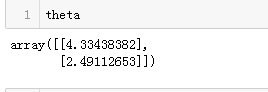
结果
theta

对批量随机下降不同步长画图
theta_path_bgd = []
def plot_gradient_descent(theta,eta,theta_path = None):
    m = len(X_b)
    plt.plot(X,y,'b.')
    n_iterations = 1000
    for iteration in range(n_iterations):
        if iteration<10:
            y_predict = X_new_b.dot(theta)
            style = 'b-' if iteration>0 else 'r--'
            plt.plot(X_new,y_predict,style)
        gradients = 2/m * X_b.T.dot(X_b.dot(theta)-y)
        theta = theta - eta * gradients
        if theta_path is not None:
            theta_path.append(theta)
    plt.xlabel('$x_1$',fontsize= 18)
    plt.axis([0,2,0,15])
    plt.title(r'$eta = {}$'.format(eta),fontsize=16)
np.random.seed(42)
theta = np.random.randn(2,1)
plt.figure(figsize=(10,4))
plt.subplot(141);plot_gradient_descent(theta,eta)
plt.ylabel("$y$", rotation=0, fontsize=18)
plt.subplot(142); plot_gradient_descent(theta, eta=0.1)
plt.subplot(143); plot_gradient_descent(theta, eta=0.5, theta_path=theta_path_bgd)
plt.subplot(144); plot_gradient_descent(theta, eta=0.6)
save_fig("gradient_descent_plot")
plt.show()
输出结果:

可以使用网格搜索寻找一个号的学习率。当然,一般会限制迭代的次数,以便网络搜索可以消除模型需要很长时间才能收敛这一问题
如何选取迭代的次数。如果它太小了,当算法停止的时候,你依然没有找到最优解。如果它太大了,算法会非常的耗时同时后来的迭代参数也不会发生改变。一个简单的解决方法是:设置一个非常大的迭代次数,但是当梯度向量变得非常小的时候,结束迭代。非常小指的是:梯度向量小于一个值 (称为容差)。这时候可以认为梯度下降几乎已经达到了最小值。
随机梯度下降
随机梯度下降由于每次的迭代只需要在内存中有一个实例,这使得随机梯度算法可以在大规模的训练集上使用,另一方面,由于他的随机性,与批量梯度下降相比,其呈现更多的不规律性:它达到最小值不是平缓的下降,损失函数忽高忽低,但总体上呈下降趋势。随着时间的推移,他会靠近最小值,但它也不会停止在某个值上,而是它会一直在这个值附近摆动。因此,当算法结束的时候,最后的参数还不错,但不是最优值。
当损失函数很不规则时,随机梯度下降算法也能够跳过局部最小值,因此,随机梯度下降在寻找全局最小值上比批量梯度下降表现要好
也正是因为随机梯度下降算法的随机性可以很好的跳过局部最优值,但同时它也不能达到最小值。解决这个问题的办法就是逐渐降低学习率:
开始时,走的每一步都比较大(这有助于快速前进并跳过局部最小值),然后变的越来越小,从而使算法达到全局最小值。这个过程称为“模拟退火”
决定每次迭代的学习率的函数称为learning schedule。如果学习速度降低的过快,可能会陷入局部最小值,甚至达到最小值的半路就停住了;如果学习速度过慢,可能在最小值的附近长时间摆动,同时如果过早停止训练,最终只会出现次优解
实现一个简单的learning schedule来实现随机梯度下降算法
n_epochs = 50
t0,t1 = 5,50

theta_path_sgd = []

def learning_schedule(t):
    return t0/(t+t1)
theta = np.random.randn(2,1)

for epoch in range(n_epochs):
    for i in range(m):
        if epoch == 0 and i < 20:
            y_predict =X_new_b.dot(theta)
            style = 'b-' if i > 0 else 'r--'
            plt.plot(X_new,y_predict,style)
        random_index = np.random.randint(m)
        xi= X_b[random_index:random_index+1]
        yi = y[random_index:random_index+1]
        gradients = 2 * xi.T.dot(xi.dot(theta) - yi)
        eta = learning_schedule(epoch*m + i)
        theta = theta - eta * gradients
        theta_path_sgd.append(theta)

plt.plot(X,y,'b.')
plt.xlabel('$x_1$',fontsize = 18)
plt.ylabel("$y$",fontsize = 18,rotation=0)
plt.axis([0,2,0,15])
plt.show()
展示第一个批次训练中前20个训练结果

theta值如下
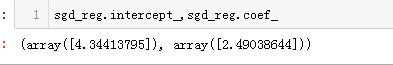
当然sklearn中也封装了该方法,可以使用SGDRegressor类完成线性回归的随机梯度下降,这个类默认优化的是均方差损失函数。这里让其迭代50次,学习率为0.1(eta0=0.1),使用默认的learning schedule(与前面的不一样),同时也没有添加任何正则项(penalty=None)
from sklearn.linear_model import SGDRegressor
sgd_reg = SGDRegressor(n_iter_no_change=50,penalty=None,eta0=0.1)
sgd_reg.fit(X,y.ravel())
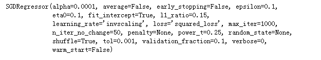
结果:
小批量梯度下降
在迭代的每一步中,批量梯度使用整个训练集,随机梯度仅仅使用了一个实例,在小批量梯度下降中,它则使用的是一个随机的小型实例集。它比随机梯度的主要优点是在于可以通过矩阵运算的硬件优化得到一个较好的训练表现
n_iterations = 50
minibatch_size = 20
theta_path_mgd = []

np.random.seed(42)
theta = np.random.randn(2,1)

t0,t1 = 200,1000
def learning_schedule(t):
    return t0/(t + t1)

t = 0
for epoch in range(n_iterations):
    shuffled_index = np.random.permutation(m)
    X_b_shuffled = X_b[shuffled_index]
    y_shuffled = y[shuffled_index]
    for i in range(0,m,minibatch_size):
        t +=1
        xi = X_b_shuffled[i:i+minibatch_size]
        yi = y_shuffled[i:i+minibatch_size]
        gradients = 2/minibatch_size * xi.T.dot(xi.dot(theta) - yi)
        eta = learning_schedule(t)
        theta = theta - eta * gradients
        theta_path_mgd.append(theta)
theta值

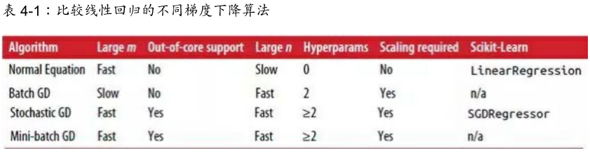
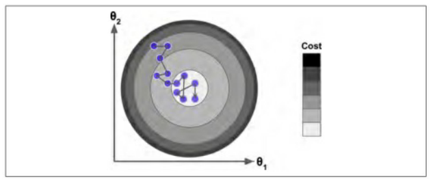
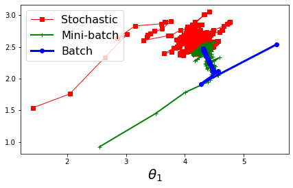
将上述三种梯度下降进行比较
参数空间的梯度下降路径展示:
代码:
plt.figure(figsize=(7,4))
plt.plot(theta_path_sgd[:,0],theta_path_sgd[:,1],'r-s',linewidth=1,label ='Stochastic')
plt.plot(theta_path_mgd[:,0],theta_path_mgd[:,1],'g-+',linewidth=2,label='Mini-batch')
plt.plot(theta_path_bgd[:,0],theta_path_bgd[:,1],'b-o',linewidth=3,label='Batch')
plt.legend(loc='upper left',fontsize=16)
plt.xlabel(r'$	heta_0$',fontsize=20)
plt.xlabel(r'$	heta_1$',fontsize=20,rotation=0)
plt.show()
比较线性回归的不同梯度下降算法: