最优化
机器学习的优化目标:最小化损失函数
梯度下降
认识梯度下降
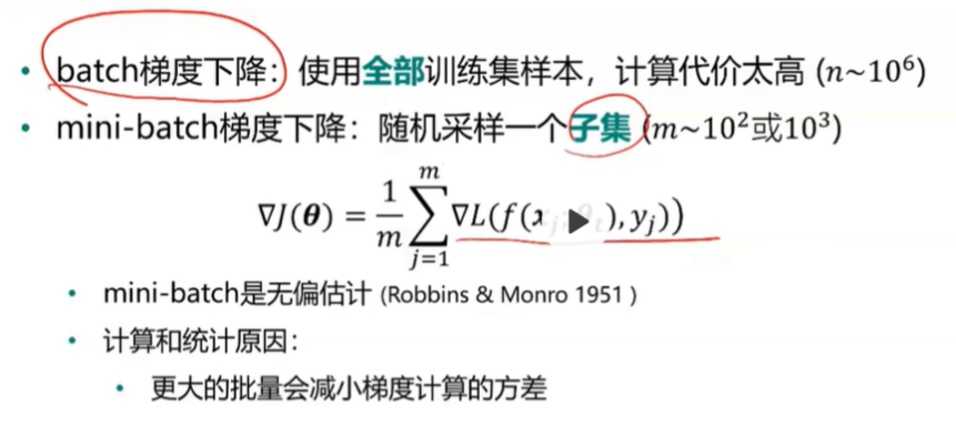
- 随机梯度下降: 使用mini-batch计算出结果后再根据梯度下降法的公式去更新参数,下一步再随机采样子集,重复该操作。此方法称为随机梯度下降(SGD)
梯度下降在实际中的问题
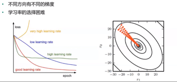
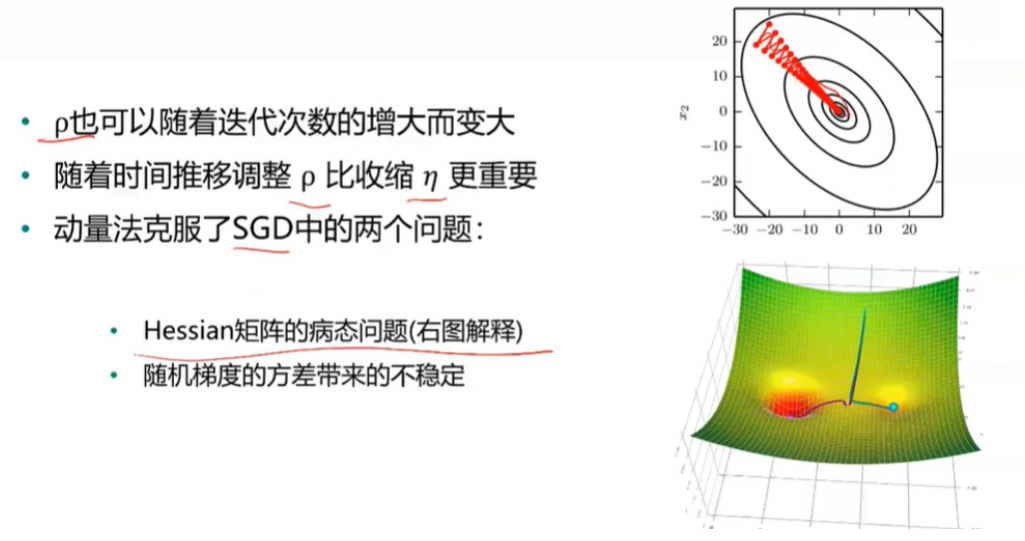
- 病态条件
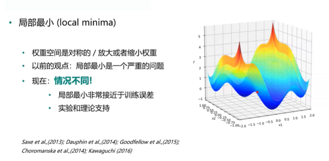
- 局部最小 VS 全局最小
SGD方法的改进
动量法
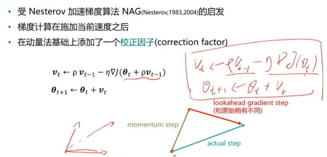
Nesterov动量法
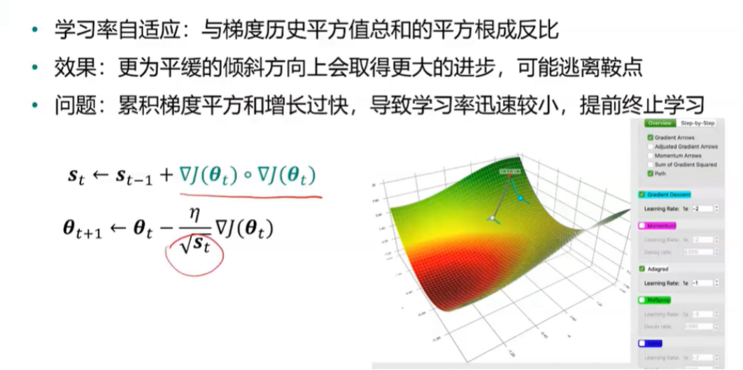
AdaGrad
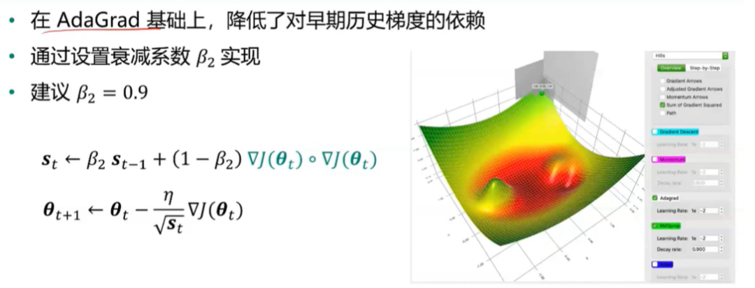
RMSProp
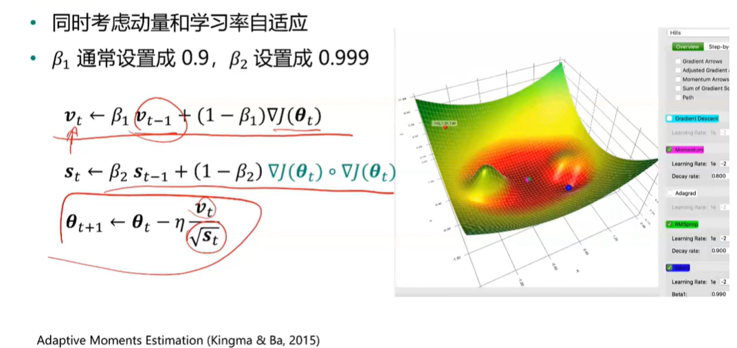
Adam
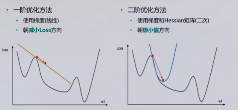
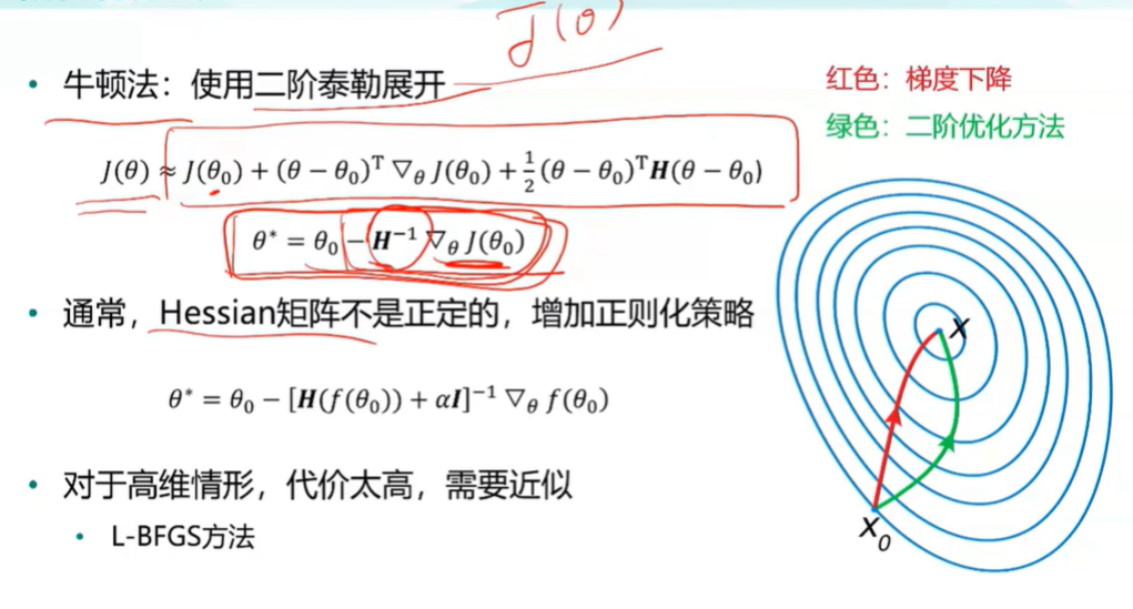
二阶优化
实例练习
#先引入算法相关的包,matplotlib用于绘图
import matplotlib.pyplot as plt
import numpy as np
from mpl_toolkits.mplot3d import Axes3D
from matplotlib import animation
from IPython.display import HTML
from autograd import elementwise_grad, value_and_grad,grad
from scipy.optimize import minimize
from scipy import optimize
from collections import defaultdict
from itertools import zip_longest
plt.rcParams['axes.unicode_minus']=False # 用来正常显示负号
#使用python的匿名函数定义目标函数
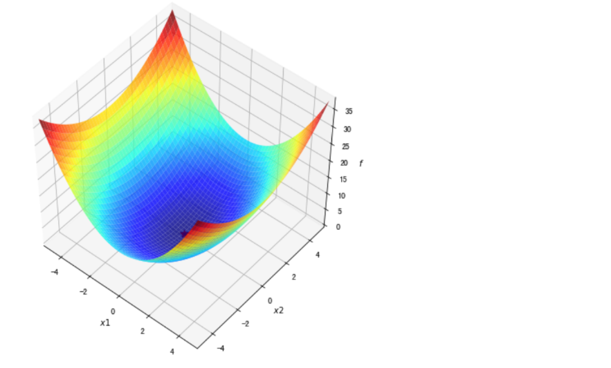
f1 = lambda x1,x2 : x1**2 + 0.5*x2**2 #函数定义
f1_grad = value_and_grad(lambda args : f1(*args)) #函数梯度
#梯度下降法
##定义gradient_descent方法对参数进行更新
###func:f1 // func_grad:f1_grad // x0:初始点 // learning_rate:学习率 // max_iteration:最大步数
def gradient_descent(func, func_grad, x0, learning_rate=0.1, max_iteration=20):
#记录该步如何走(可视化使用)
path_list = [x0]
#当前走到哪个位置
best_x = x0
step = 0
while step < max_iteration:
update = -learning_rate * np.array(func_grad(best_x)[1])
if(np.linalg.norm(update) < 1e-4):
break
best_x = best_x + update
path_list.append(best_x)
step = step + 1
return best_x, np.array(path_list)
#绘制函数曲面
##先借助np.meshgrid生成网格点坐标矩阵。两个维度上每个维度显示范围为-5到5。对应网格点的函数值保存在z中
x1,x2 = np.meshgrid(np.linspace(-5.0,5.0,50), np.linspace(-5.0,5.0,50))
z = f1(x1,x2 )
minima = np.array([0, 0]) #对于函数f1,我们已知最小点为(0,0)
ax.plot_surface?
##plot_surface函数绘制3D曲面
%matplotlib inline
fig = plt.figure(figsize=(8, 8))
ax = plt.axes(projection='3d', elev=50, azim=-50)
ax.plot_surface(x1,x2, z, alpha=.8, cmap=plt.cm.jet)
ax.plot([minima[0]],[minima[1]],[f1(*minima)], 'r*', markersize=10)
ax.set_xlabel('$x1$')
ax.set_ylabel('$x2$')
ax.set_zlabel('$f$')
ax.set_xlim((-5, 5))
ax.set_ylim((-5, 5))
plt.show()
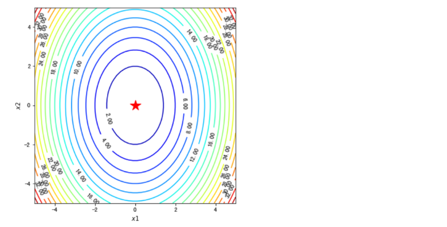
#绘制等高线和梯度场
##contour方法能够绘制等高线,clabel能够将对应线的高度(函数值)显示出来,这里我们保留两位小数(fmt='%.2f')。
dz_dx1 = elementwise_grad(f1, argnum=0)(x1, x2)
dz_dx2 = elementwise_grad(f1, argnum=1)(x1, x2)
fig, ax = plt.subplots(figsize=(6, 6))

contour = ax.contour(x1, x2, z,levels=20,cmap=plt.cm.jet)
ax.clabel(contour,fontsize=10,colors='k',fmt='%.2f')
ax.plot(*minima, 'r*', markersize=18)

ax.set_xlabel('$x1$')
ax.set_ylabel('$x2$')

ax.set_xlim((-5, 5))
ax.set_ylim((-5, 5))

plt.show()
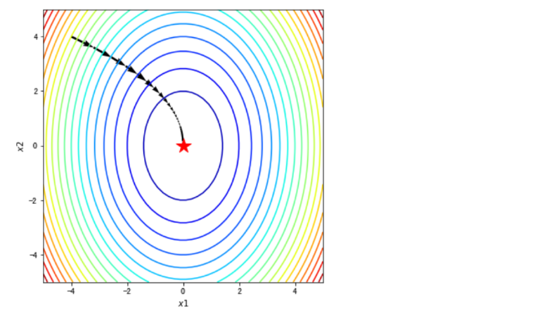
#在梯度场内使用quiver函数将路径画出来
fig, ax = plt.subplots(figsize=(6, 6))

ax.contour(x1, x2, z, levels=20,cmap=plt.cm.jet)#等高线
#绘制轨迹箭头
ax.quiver(path_list_gd[:-1,0], path_list_gd[:-1,1], path_list_gd[1:,0]-path_list_gd[:-1,0], path_list_gd[1:,1]-path_list_gd[:-1,1], scale_units='xy', angles='xy', scale=1, color='k')
#标注最优值点
ax.plot(*minima, 'r*', markersize=18)

ax.set_xlabel('$x1$')
ax.set_ylabel('$x2$')

ax.set_xlim((-5, 5))
ax.set_ylim((-5, 5))
plt.show()
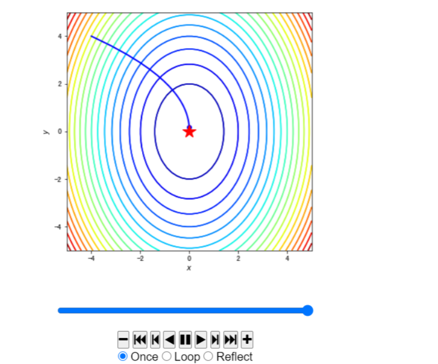
#使用animation动画化
path = path_list_gd #梯度下降法的优化路径
fig, ax = plt.subplots(figsize=(6, 6))
line, = ax.plot([], [], 'b', label='Gradient Descent', lw=2) #保存路径
point, = ax.plot([], [], 'bo') #保存路径最后的点
#最开始画什么
def init_draw():
    ax.contour(x1, x2, z, levels=20, cmap=plt.cm.jet)
    ax.plot(*minima, 'r*', markersize=18) #将最小值点绘制成红色五角星
    ax.set_xlabel('$x$')
    ax.set_ylabel('$y$')
    ax.set_xlim((-5, 5))
    ax.set_ylim((-5, 5))
    return line, point
#每一步更新画什么
def update_draw(i):
    line.set_data(path[:i,0],path[:i,1])
    point.set_data(path[i-1:i,0],path[i-1:i,1])
    plt.close()
    return line, point

anim = animation.FuncAnimation(fig, update_draw, init_func=init_draw,frames=path.shape[0], interval=60, repeat_delay=5, blit=True)
HTML(anim.to_jshtml())