1 Statistical Learning
1.1 What Is Statistical Learning?
More generally, suppose that we observe a quantitative response Y and p different predictors, X1,X2, . . .,Xp. We assume that there is some relationship between Y and X = (X1,X2, . . .,Xp), which can be written in the very general form
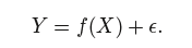
Statistical learning refers to a set of approaches for estimating f.
1.1.1 Why Estimate f?
Prediction(预测) and inference(推断).
1. Prediction
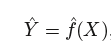
where ˆ f represents our estimate for f, and ˆ Y represents the resulting prediction for Y.
^ f is often treated as a black box.
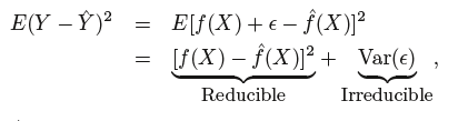
The accuracy of ˆ Y as a prediction for Y depends on two quantities, which we will call the reducible error(可约误差) and the irreducible error(不可约误差).
reducible error: In general, “^f will not be a perfect estimate for f, and this inaccuracy will introduce some error. This error is reducible because we can potentially improve the accuracy of ˆ f by using the most appropriate statistical learning technique to estimate f
irreducible error: Y is also a function of ϵ, which, by definition, cannot be predicted using X. Therefore, variability associated with ϵ also affects the accuracy of our prediction.
2. Inference
To understand the relationship between X and Y , or more specifically, to understand how Y changes as a function of X1, . . .,Xp. Now ˆ f cannot be treated as a black box, because we need to know its exact form.
1.1.2 How Do We Estimate f?
1. Parametric methods(参数方法)
Parametric methods involve a two-step model-based approach.
(1) First, we make an assumption about the functional form, or shape, of f. For example, one very simple assumption is that f is linear in X:
(2) After a model has been selected, we need a procedure that uses the training data to fit or train the model
Advantage: simplifies the problem
Disadvantage: The potential disadvantage of a parametric approach is that the model we choose will usually not match the true unknown form of f. If the chosen model is too far from the true f, then our estimate will be poor.
2. Non-parametric Methods(非参数方法)
Non-parametric methods do not make explicit assumptions about the functional form of f.
Advantage: by avoiding the assumption of a particular functional form for f, they have the potential to accurately fit a wider range of possible shapes for f.
Disadvantage: since they do not reduce the problem of estimating f to a small number of parameters, a very large number of observations (far more than is typically needed for a parametric approach) is required in order to obtain an accurate estimate for f
1.1.3 The Trade-Off Between Prediction Accuracy and Model Interpretability(预测精度和模型解释性的权衡)
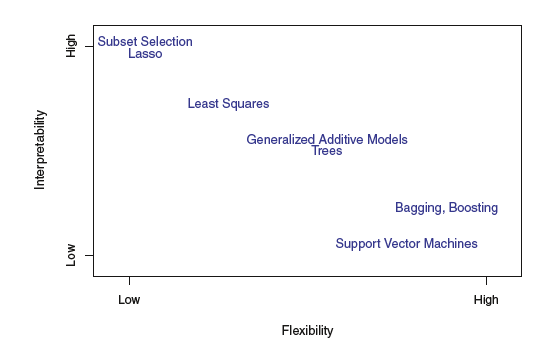
We have established that when inference is the goal, there are clear advantages to using simple and relatively inflexible statistical learning methods. Surprisingly, we will often obtain more accurate predictions using a less flexible method.
1.3.4 Supervised Versus Unsupervised Learning
1. Supervised Learning
For each observation of the predictor measurement(s) xi, i = 1, …, n there is an associated response measurement yi. Such as linear regression and logistic regression, GAM, boosting, and support vector machines
2. Unsupervised Learning
Unsupervised learning describes the somewhat more challenging situation in which for every observation i = 1, . . . , n, we observe a vector of measurements xi but no associated response yi. Such as cluster analysis.
1.2Assessing Model Accuracy(模型精度评价)
1.2.1 Measuring the Quality of Fit(拟合效果检验)
mean squared error (MSE):
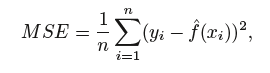
where ˆ f(xi) is the prediction that ˆ f gives for the ith observation
training MSE(训练均方误差):The MSE is computed using the training data that was used to fit the model
test MSE(测试均方误差):
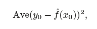 测试均方误差越小越好
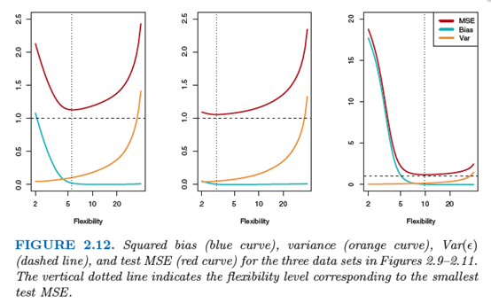
1.2.2 The Bias-Variance Trade-Off(偏差一方差权衡)
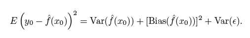
Variance refers to the amount by which ˆ f would change if we estimated it using a different training data set.
Bias refers to the error that is introduced by approximating a real-life problem, which may be extremely complicated, by a much simpler model.
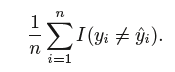
1.2.3 The Classification Setting
training error rate:
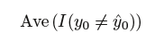
test error rate:
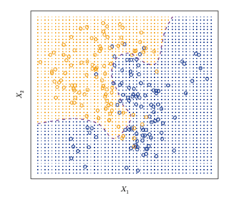
1. The Bayes Classifier
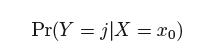
In a two-class problem where there are Bayes only two possible response values, say class 1 or class 2, the Bayes classifier corresponds to predicting class one if Pr(Y = 1|X = x0) > 0.5, and class two otherwise.
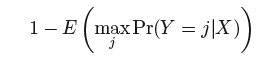
the overall Bayes error rate is given by
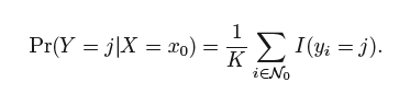
2. K-Nearest Neighbors
Given a positive integer K and a test observation x0, the KNN classifier first identifies the neighbors K points in the training data that are closest to x0, represented by N0. It then estimates the conditional probability for class j as the fraction of points in N0 whose response values equal j: