python机器学习-乳腺癌细胞挖掘(博主亲自录制视频)

项目合作QQ:231469242
fisher's exact test算法来自超几何分布


python代码
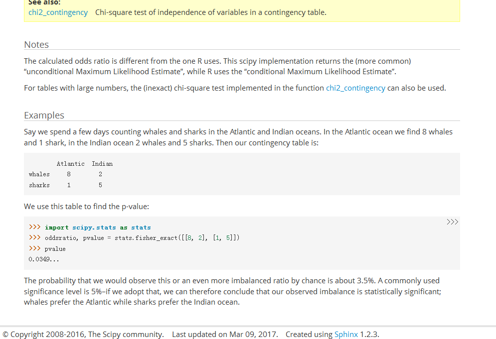
https://docs.scipy.org/doc/scipy/reference/generated/scipy.stats.fisher_exact.html

在线工具
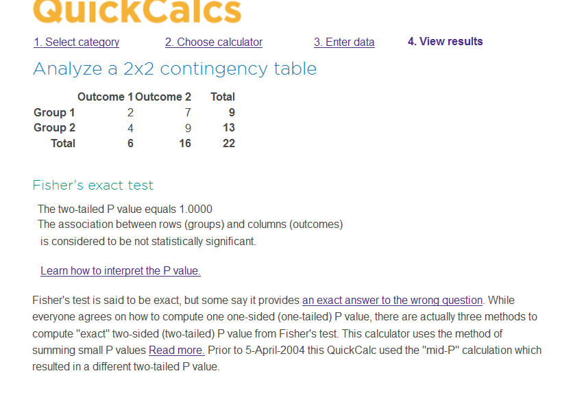
graphpad公司已经把桌面软件做成网页版本。fisher's exact test和卡方类似,但准确性更高,因为卡方分析的p是估计值,不是准确值。除非某人指定你用卡方分析,否则用fisher's exact test。推荐用双边检查。
http://graphpad.com/quickcalcs/contingency1/


计算结果
维基百科解释
https://en.wikipedia.org/wiki/Fisher's_exact_test
Fisher's exact test is a statistical significance test used in the analysis of contingency tables.[1][2][3] Although in practice it is employed when sample sizes are small, it is valid for all sample sizes. It is named after its inventor, Ronald Fisher, and is one of a class of exact tests, so called because the significance of the deviation from a null hypothesis (e.g., P-value) can be calculated exactly, rather than relying on an approximation that becomes exact in the limit as the sample size grows to infinity, as with many statistical tests.
Fisher is said to have devised the test following a comment from Dr. Muriel Bristol, who claimed to be able to detect whether the tea or the milk was added first to her cup. He tested her claim in the "lady tasting tea" experiment.[4]
Purpose and scope

The test is useful for categorical data that result from classifying objects in two different ways; it is used to examine the significance of the association (contingency) between the two kinds of classification. So in Fisher's original example, one criterion of classification could be whether milk or tea was put in the cup first; the other could be whether Dr. Bristol thinks that the milk or tea was put in first. We want to know whether these two classifications are associated—that is, whether Dr. Bristol really can tell whether milk or tea was poured in first. Most uses of the Fisher test involve, like this example, a 2 × 2 contingency table. The p-value from the test is computed as if the margins of the table are fixed, i.e. as if, in the tea-tasting example, Dr. Bristol knows the number of cups with each treatment (milk or tea first) and will therefore provide guesses with the correct number in each category. As pointed out by Fisher, this leads under a null hypothesis of independence to a hypergeometric distribution of the numbers in the cells of the table.
With large samples, a chi-squared test can be used in this situation. However, the significance value it provides is only an approximation, because the sampling distribution of the test statistic that is calculated is only approximately equal to the theoretical chi-squared distribution. The approximation is inadequate when sample sizes are small, or the data are very unequally distributed among the cells of the table, resulting in the cell counts predicted on the null hypothesis (the “expected values”) being low. The usual rule of thumb for deciding whether the chi-squared approximation is good enough is that the chi-squared test is not suitable when the expected values in any of the cells of a contingency table are below 5, or below 10 when there is only one degree of freedom (this rule is now known to be overly conservative[5]). In fact, for small, sparse, or unbalanced data, the exact and asymptotic p-values can be quite different and may lead to opposite conclusions concerning the hypothesis of interest.[6][7] In contrast the Fisher exact test is, as its name states, exact as long as the experimental procedure keeps the row and column totals fixed, and it can therefore be used regardless of the sample characteristics. It becomes difficult to calculate with large samples or well-balanced tables, but fortunately these are exactly the conditions where the chi-squared test is appropriate.
For hand calculations, the test is only feasible in the case of a 2 × 2 contingency table. However the principle of the test can be extended to the general case of an m × n table,[8][9] and some statistical packages provide a calculation (sometimes using a Monte Carlo method to obtain an approximation) for the more general case.[10]
Example
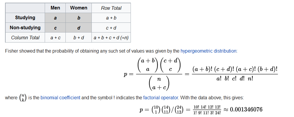
For example, a sample of teenagers might be divided into male and female on the one hand, and those that are and are not currently studying for a statistics exam on the other. We hypothesize, for example, that the proportion of studying individuals is higher among the women than among the men, and we want to test whether any difference of proportions that we observe is significant. The data might look like this:
| Men | Women | Row total | |
|---|---|---|---|
| Studying | 1 | 9 | 10 |
| Not-studying | 11 | 3 | 14 |
| Column total | 12 | 12 | 24 |
The question we ask about these data is: knowing that 10 of these 24 teenagers are studiers, and that 12 of the 24 are female, and assuming the null hypothesis that men and women are equally likely to study, what is the probability that these 10 studiers would be so unevenly distributed between the women and the men? If we were to choose 10 of the teenagers at random, what is the probability that 9 or more of them would be among the 12 women, and only 1 or fewer from among the 12 men?
Before we proceed with the Fisher test, we first introduce some notations. We represent the cells by the letters a, b, c and d, call the totals across rows and columns marginal totals, and represent the grand total by n. So the table now looks like this:
| Men | Women | Row Total | |
|---|---|---|---|
| Studying | a | b | a + b |
| Non-studying | c | d | c + d |
| Column Total | a + c | b + d | a + b + c + d (=n) |
Fisher showed that the probability of obtaining any such set of values was given by the hypergeometric distribution:

where
 is the

The formula above gives the exact hypergeometric probability of observing this particular arrangement of the data, assuming the given marginal totals, on the null hypothesis that men and women are equally likely to be studiers. To put it another way, if we assume that the probability that a man is a studier is P, the probability that a woman is a studier is p, and we assume that both men and women enter our sample independently of whether or not they are studiers, then this hypergeometric formula gives the conditional probability of observing the values a, b, c, d in the four cells, conditionally on the observed marginals (i.e., assuming the row and column totals shown in the margins of the table are given). This remains true even if men enter our sample with different probabilities than women. The requirement is merely that the two classification characteristics—gender, and studier (or not)—are not associated.
For example, suppose we knew probabilities
 with
with  such that (male studier, male non-studier, female studier, female non-studier) had respective probabilities
  for each individual encountered under our sampling procedure. Then still, were we to calculate the distribution of cell entries conditional given marginals, we would obtain the above formula in which neither p nor P occurs. Thus, we can calculate the exact probability of any arrangement of the 24 teenagers into the four cells of the table, but Fisher showed that to generate a significance level, we need consider only the cases where the marginal totals are the same as in the observed table, and among those, only the cases where the arrangement is as extreme as the observed arrangement, or more so. (
| Men | Women | Row Total | |
|---|---|---|---|
| Studying | 0 | 10 | 10 |
| Non-studying | 12 | 2 | 14 |
| Column Total | 12 | 12 | 24 |
For this table (with extremely unequal studying proportions) the probability is
 .
.In order to calculate the significance of the observed data, i.e. the total probability of observing data as extreme or more extreme if the null hypothesis is true, we have to calculate the values of p for both these tables, and add them together. This gives a one-tailed test, with p approximately 0.001346076 + 0.000033652 = 0.001379728. For example, in the R statistical computing environment, this value can be obtained as fisher.test(rbind(c(1,9),c(11,3)), alternative="less")$p.value. This value can be interpreted as the sum of evidence provided by the observed data—or any more extreme table—for the null hypothesis (that there is no difference in the proportions of studiers between men and women). The smaller the value of p, the greater the evidence for rejecting the null hypothesis; so here the evidence is strong that men and women are not equally likely to be studiers.
For a two-tailed test we must also consider tables that are equally extreme, but in the opposite direction. Unfortunately, classification of the tables according to whether or not they are 'as extreme' is problematic. An approach used by the fisher.test function in R is to compute the p-value by summing the probabilities for all tables with probabilities less than or equal to that of the observed table. In the example here, the 2-sided p-value is twice the 1-sided value—but in general these can differ substantially for tables with small counts, unlike the case with test statistics that have a symmetric sampling distribution.
As noted above, most modern statistical packages will calculate the significance of Fisher tests, in some cases even where the chi-squared approximation would also be acceptable. The actual computations as performed by statistical software packages will as a rule differ from those described above, because numerical difficulties may result from the large values taken by the factorials. A simple, somewhat better computational approach relies on a gamma function or log-gamma function, but methods for accurate computation of hypergeometric and binomial probabilities remains an active research area.
Controversies
Despite the fact that Fisher's test gives exact p-values, some authors have argued that it is conservative, i.e. that its actual rejection rate is below the nominal significance level.[11][12][13] The apparent contradiction stems from the combination of a discrete statistic with fixed significance levels.[14][15] To be more precise, consider the following proposal for a significance test at the 5%-level: reject the null hypothesis for each table to which Fisher's test assigns a p-value equal to or smaller than 5%. Because the set of all tables is discrete, there may not be a table for which equality is achieved. If
 is the largest p-value smaller than 5% which can actually occur for some table, then the proposed test effectively tests at the
 The decision to condition on the margins of the table is also controversial.[17][18] The p-values derived from Fisher's test come from the distribution that conditions on the margin totals. In this sense, the test is exact only for the conditional distribution and not the original table where the margin totals may change from experiment to experiment. It is possible to obtain an exact p-value for the 2x2 table when the margins are not held fixed. Barnard's test, for example, allows for random margins. However, some authors[14][15][18] (including, later, Barnard himself)[14] have criticized Barnard's test based on this property. They argue that the marginal success total is an (almost[15]) ancillary statistic, containing (almost) no information about the tested property.
The act of conditioning on the marginal success rate from a 2x2 table can be shown to ignore some information in the data about the unknown odds ratio.[19] The argument that the marginal totals are (almost) ancillary implies that the appropriate likelihood function for making inferences about this odds ratio should be conditioned on the marginal success rate.[19] Whether this lost information is important for inferential purposes is the essence of the controversy.[19]
Alternatives
An alternative exact test, Barnard's exact test, has been developed and proponents of it suggest that this method is more powerful, particularly in 2 × 2 tables. Another alternative is to use maximum likelihood estimates to calculate a p-value from the exact binomial or multinomial distributions and reject or fail to reject based on the p-value.[citation needed]
For stratified categorical data the Cochran–Mantel–Haenszel test must be used instead of Fisher's test.
Choi et al.[19] propose a p-value derived from the likelihood ratio test based on the conditional distribution of the odds ratio given the marginal success rate. This p-value is inferentially consistent with classical tests of normally distributed data as well as with likelihood ratios and support intervals based on this conditional likelihood function. It is also readily computable.[20]
See also
http://blog.sina.com.cn/s/blog_5ecfd9d90100oa4c.html
并没有自己写,看了一篇小短文,觉得不错,直接拿来了。
引自----應數博黃士峰
費雪(R. A. Fisher, 1890-1962, 英國統計學家)在他1935 年發表的一篇文章
中提到一個有趣的實驗。有一天喝下午茶時,費雪的一位女同事說到,下午茶的
調製順序對其風味有很大的影響,把茶加進牛奶裡或者是把牛奶倒入茶中,兩者
喝起來口感完全不同,她可以完全地分辨出來,而她個人的偏好是先放牛奶再加
入茶。為了證實這位女同事的說法,費雪做了ㄧ個小實驗。首先他調製了8 杯下
午茶,並且告訴女同事其中4 杯是先放牛奶再加入茶,另外4 杯則是先倒茶再加
入牛奶,接著費雪隨機的拿了一杯茶讓女同事試喝,並請她猜猜這杯茶中是先放
牛奶還是先放茶,等女同事回答後,再隨機的拿第二杯請她試喝,直到全部試喝
完畢。假設女同事的答案如下表:
實際先放的飲料 牛奶 茶 合計
牛奶 a = 3 b = 1 a+b = 4
茶 c = 1 d = 3 c+d = 4
合計 a+c = 4 b+d = 4 n = 8
由表中得知費雪的女同事猜對了6 杯,但這是否只是碰巧她當天運氣好呢?能否
以統計方法讓我們由實驗的數據判斷費雪的女同事能否真的分辨出兩種不同的
下午茶調製方法?另一個值得注意的事情是,在這個實驗中樣本數非常的小,是
否有適當的統計方法可以幫助我們做出統計推論呢?
對於以上的問題, 費雪在1935 的文章中提出一個小樣本的檢定方法,稱為
Fisher’s Exact Test。這個方法的前提是固定邊際分布,也就是a+b 、c+d、a+c、
與b+d 的值不變,接著計算在此假設下,得到實際觀測值的機率:
p(a=3|a+b=c+d=a+c=b+d=4)=0.229
其中P(A | B) 是在B 事件發生的前提下A 事件發生的條件機率.
。這個數值的意義是如果費雪的女同事只是隨便亂猜的話,最後
會得到上述表格中結果的機率為0.229。接著我們可更進一步的算出比表格中更
極端情況( 在此指費雪的女同事猜得更準時) 的機率:
P(a = 4 | a + b = c + d = a + c = b + d = 4) = 0.014 , 因此我們可以再計算出
P(a ≥ 3 | a + b = c + d = a + c = b + d = 4) = 0.229 + 0.014 = 0.243 ,此即為統計上單
邊檢定的p 值(p-value)。如果此p 值小於型一誤的機率(the probability of type one
error,一般常設定為0.05 或0.01),則我們可以說有充分的證據支持費雪的女同
事所言不虛,反之則是證據仍不足以證實她的說法。費雪在1935 年的文章中並
沒有告訴我們當時這位女同事到底猜對了幾杯,但根據費雪女兒後來的說法是,
這位女同事當時全答對了(Agresti 2002, p.92)。
上述的小故事看起來好像只是一則有趣的實驗,對統計的實際應用有什麼影
響呢?實際上,Fisher’s Exact Test 不僅簡單實用,尤其適用於樣本數小的情況,
而且這個方法並不需要假設資料母體的分布,換句話說,Fisher’s Exact Test 屬於
一種無母數的檢定方法。以下再舉幾個實際應用的例子:
一、 現在大學生流行節食,一般大眾的猜測是:大學女生節食的比例比男生高。
因此我們設定的虛無假設為H0:大學女生與男生節食的比例相同,對立假
設為Ha:大學女生節食的比例比男生高。倘若經過調查後我們得到以下的
資料:
男生 女生 合計
節食 a = 1 b = 9 a+b = 10
未節食 c = 11 d = 3 c+d = 14
合計 a+c = 12 b+d = 12 n = 24
則我們可根據上表中的資料算出單邊檢定的p 值
0.0014.
若設定型一誤的機率為0.01,則我們可根據此p 值推論:上表中的資料提
供了足夠的證據拒絕虛無假設,並支持對立假設,即大學女生節食的比例
比男生高。
二、 某家醫院統計了罹患某種罕見疾病時,男性與女性的死亡與存活資料如下:
男性 女性 合計
存活 a = 9 b = 4 a+b = 13
死亡 c = 1 d = 10 c+d = 11
合計 a+c = 10 b+d = 14 n = 24
根據上表,女性死亡率似乎遠比男性為高,因此設定虛無假設為H0:女性
與男性患者死亡率相同,對立假設為Ha:女性患者死亡率較男性高。則我
們可根據上表中的資料算出單邊檢定的p 值
0.0042.
若設定型一誤的機率為0.01,則我們可根據此p 值推論:女性患者死亡率
較男性高。
參考文獻
Agresti, A. (2002). Categorical Data Analysis. John Wiley, New Jersey.
Fisher, R. A. (1935). The Design of Experiments. Oliver & Boyd, Edinburgh.
另外,wiki上解释的也很好:
Fisher's exact test[1][2][3] is a statistical significance test used in the analysis of contingency tables where sample sizes are small. It is named after its inventor, R. A. Fisher, and is one of a class of exact tests, so called because the significance of the deviation from a null hypothesis can be calculated exactly, rather than relying on an approximation that becomes exact in the limit as the sample size grows to infinity, as with many statistical tests. Fisher is said to have devised the test following a comment from Muriel Bristol, who claimed to be able to detect whether the tea or the milk was added first to her cup; see lady tasting tea.

import scipy.stats as stats
stats.fisher_exact(obs)
Out[3]: (20.0, 0.034965034965034919)

stats.chi2_contingency(obs)
Out[4]:
(3.8095238095238093, 0.050961936967763424, 1, array([[ 5.625,  4.375],
        [ 3.375,  2.625]]))

| Men | Women | Row total | |
|---|---|---|---|
| Studying | 1 | 9 | 10 |
| Not-studying | 11 | 3 | 14 |
| Column total | 12 | 12 | 24 |
obs = np.array([[1, 9], [11, 3]])

stats.fisher_exact(obs)
Out[7]: (0.030303030303030304, 0.002759456185220084)

stats.chi2_contingency(obs)
Out[8]:
(8.4000000000000004, 0.0037522101008738498, 1, array([[ 5.,  5.],
        [ 7.,  7.]]))
猜測先放的飲料
實際先放的飲料
牛奶
茶
合計
牛奶
a =
3
b =
1
a+b = 4
茶
c =
1
d =
3
c+d = 4
合計
a+c = 4 b+d =
4
n = 8
obs = np.array([[3,1], [1, 3]])

stats.fisher_exact(obs)
Out[14]: (9.0, 0.48571428571428543)

stats.chi2_contingency(obs)
Out[15]:
(0.5, 0.47950012218695337, 1, array([[ 2.,  2.],
        [ 2.,  2.]]))
男生 女生 合計
節食 a =
1
b = 9 a+b = 10
未節食 c =
11
d = 3 c+d =
14
合計
a+c = 12 b+d = 12 n = 24
卡方和Fisher检测表示都有显著关系
obs = np.array([[1,9], [11, 3]])

stats.fisher_exact(obs)
Out[17]: (0.030303030303030304, 0.002759456185220084)

stats.chi2_contingency(obs)
Out[18]:
(8.4000000000000004, 0.0037522101008738498, 1, array([[ 5.,  5.],
        [ 7.,  7.]]))
https://study.163.com/provider/400000000398149/index.htm?share=2&shareId=400000000398149( 欢迎关注博主主页,学习python视频资源,还有大量免费python经典文章)