从0到1Python数据科学之旅(博主录制)
http://dwz.date/cqpw

本文作为学术探讨,介绍逐步回归原理和python代码。当基于最小二乘法训练线性回归模型而发生过拟合现象时,最小二乘法没有办法阻止学习过程。前向逐步回归的引入则可以控制学习过程中出现的过拟合,它是最小二乘法的一种改进或者说调整,其基本思想是由少到多地向模型中引入变量,每次增加一个,直到没有可以引入的变量为止。最后通过比较在预留样本上计算出的错误进行模型的选择。
实现代码如下:
# 导入要用到的各种包和函数
import numpy as np
import pandas as pd
from sklearn import datasets, linear_model
from math import sqrt
import matplotlib.pyplot as plt
# 读入要用到的红酒数据集
wine_data = pd.read_csv('wine.csv')
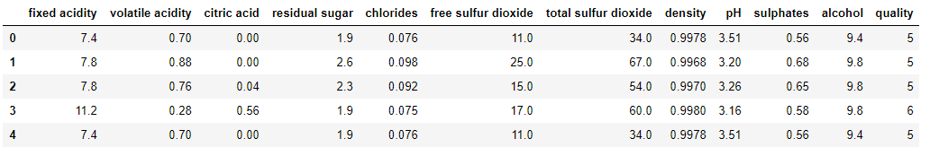
wine_data.head()
wine_data的表结构如下图所示:
# 查看红酒数据集的统计信息
wine_data.describe(
wine_data中部分属性的统计信息如下:

# 定义从输入数据集中取指定列作为训练集和测试集的函数(从取1列一直到取11列):
def xattrSelect(x, idxSet):
    xOut = []
    for row in x:
        xOut.append([row[i] for i in idxSet])
    return(xOut)


xList = []  # 构造用于存放属性集的列表
labels = [float(label) for label in wine_data.iloc[:,-1].tolist()]  # 提取出wine_data中的标签集并放入列表中
names = wine_data.columns.tolist()          # 提取出wine_data中所有属性的名称并放入列表中
for i in range(len(wine_data)):
    xList.append(wine_data.iloc[i,0:-1])    # 列表xList中的每个元素对应着wine_data中除去标签列的每一行

# 将原始数据集划分成训练集(占2/3)和测试集(占1/3):
indices = range(len(xList))
xListTest = [xList[i] for i in indices if i%3 == 0 ]
xListTrain = [xList[i] for i in indices if i%3 != 0 ]
labelsTest = [labels[i] for i in indices if i%3 == 0]
labelsTrain = [labels[i] for i in indices if i%3 != 0]


attributeList = []            # 构造用于存放属性索引的列表
index = range(len(xList[1]))  # index用于下面代码中的外层for循环
indexSet = set(index)         # 构造由names中的所有属性对应的索引构成的索引集合
oosError = []                 # 构造用于存放下面代码中的内层for循环每次结束后最小的RMSE


for i in index:
    attSet = set(attributeList)
    attTrySet = indexSet - attSet          # 构造由不在attributeList中的属性索引组成的集合
    attTry = [ii for ii in attTrySet]      # 构造由在attTrySet中的属性索引组成的列表
    errorList = []
    attTemp = []

    for iTry in attTry:
        attTemp = [] + attributeList
        attTemp.append(iTry)

        # 调用attrSelect函数从xListTrain和xListTest中选取指定的列构成暂时的训练集与测试集
        xTrainTemp = xattrSelect(xListTrain, attTemp)
        xTestTemp = xattrSelect(xListTest, attTemp)

        # 将需要用到的训练集和测试集都转化成数组对象
        xTrain = np.array(xTrainTemp)
        yTrain = np.array(labelsTrain)
        xTest = np.array(xTestTemp)
        yTest = np.array(labelsTest)

        # 使用scikit包训练线性回归模型
        wineQModel = linear_model.LinearRegression()
        wineQModel.fit(xTrain,yTrain)

        # 计算在测试集上的RMSE
        rmsError = np.linalg.norm((yTest-wineQModel.predict(xTest)), 2)/sqrt(len(yTest)) # 利用向量的2范数计算RMSE
        errorList.append(rmsError)
        attTemp = []

    iBest = np.argmin(errorList)          # 选出errorList中的最小值对应的新索引
    attributeList.append(attTry[iBest])   # 利用新索引iBest将attTry中对应的属性索引添加到attributeList中
    oosError.append(errorList[iBest])     # 将errorList中的最小值添加到oosError列表中

print("Out of sample error versus attribute set size" )
print(oosError)
print("
" + "Best attribute indices")
print(attributeList)
namesList = [names[i] for i in attributeList]
print("
" + "Best attribute names")
print(namesList)
上述代码的输出结果为:
Out of sample error versus attribute set size
[0.7234259255146811, 0.6860993152860264, 0.6734365033445415, 0.6677033213922949,
0.6622558568543597, 0.6590004754171893, 0.6572717206161052, 0.6570905806225685,
0.6569993096464123, 0.6575818940063175, 0.6573909869028242]

Best attribute indices
[10, 1, 9, 4, 6, 8, 5, 3, 2, 7, 0]

Best attribute names
['alcohol', 'volatile acidity', 'sulphates', 'chlorides', 'total sulfur dioxide', 'pH',
'free sulfur dioxide', 'residual sugar', 'citric acid', 'density', 'fixed acidity']
# 绘制由不同数量的属性构成的线性回归模型在测试集上的RMSE与属性数量的关系图像
x = range(len(oosError))
plt.plot(x, oosError, 'k')
plt.xlabel('Number of Attributes')
plt.ylabel('Error (RMS)')
plt.show()

# 绘制由最佳数量的属性构成的线性回归模型在测试集上的误差分布直方图
indexBest = oosError.index(min(oosError))
attributesBest = attributeList[1:(indexBest+1)]   # attributesBest包含8个属性索引

# 调用xattrSelect函数从xListTrain和xListTest中选取最佳数量的列组成暂时的训练集和测试集
xTrainTemp = xattrSelect(xListTrain, attributesBest)
xTestTemp = xattrSelect(xListTest, attributesBest)
xTrain = np.array(xTrainTemp)    # 将xTrain转化成数组对象
xTest = np.array(xTestTemp)      # 将xTest转化成数组对象

# 训练模型并绘制直方图
wineQModel = linear_model.LinearRegression()
wineQModel.fit(xTrain,yTrain)
errorVector = yTest-wineQModel.predict(xTest)
plt.hist(errorVector)
plt.xlabel("Bin Boundaries")
plt.ylabel("Counts")
plt.show()

# 绘制红酒口感实际值与预测值之间的散点图
plt.scatter(wineQModel.predict(xTest), yTest, s=100, alpha=0.10)
plt.xlabel('Predicted Taste Score')
plt.ylabel('Actual Taste Score')
plt.show()
上述代码绘制的图像如下:
RMSE与属性数量的关系图像:

错误直方图:

实际值与预测值的散点图:

逐步回归练习和代码
from sklearn.datasets import load_boston
import pandas as pd
import numpy as np
import statsmodels.api as sm

data = load_boston()
X = pd.DataFrame(data.data, columns=data.feature_names)
y = data.target

def stepwise_selection(X, y,
                       initial_list=[],
                       threshold_in=0.01,
                       threshold_out = 0.05,
                       verbose = True):
    """ Perform a forward-backward feature selection
    based on p-value from statsmodels.api.OLS
    Arguments:
        X - pandas.DataFrame with candidate features
        y - list-like with the target
        initial_list - list of features to start with (column names of X)
        threshold_in - include a feature if its p-value < threshold_in
        threshold_out - exclude a feature if its p-value > threshold_out
        verbose - whether to print the sequence of inclusions and exclusions
    Returns: list of selected features
    Always set threshold_in < threshold_out to avoid infinite looping.
    See https://en.wikipedia.org/wiki/Stepwise_regression for the details
    """
    included = list(initial_list)

    while True:
        changed=False
        # forward step
        excluded = list(set(X.columns)-set(included))
        new_pval = pd.Series(index=excluded)
        for new_column in excluded:
            model = sm.OLS(y, sm.add_constant(pd.DataFrame(X[included+[new_column]]))).fit()
            new_pval[new_column] = model.pvalues[new_column]
        best_pval = new_pval.min()
        if best_pval < threshold_in:
            best_feature = new_pval.argmin()
            included.append(best_feature)
            changed=True
            if verbose:
                print('Add  {:30} with p-value {:.6}'.format(best_feature, best_pval))
        # backward step
        model = sm.OLS(y, sm.add_constant(pd.DataFrame(X[included]))).fit()
        # use all coefs except intercept
        pvalues = model.pvalues.iloc[1:]
        worst_pval = pvalues.max() # null if pvalues is empty
        if worst_pval > threshold_out:
            changed=True
            worst_feature = pvalues.argmax()
            included.remove(worst_feature)
            if verbose:
                print('Drop {:30} with p-value {:.6}'.format(worst_feature, worst_pval))
        if not changed:
            break
    return included

result = stepwise_selection(X, y)

print('resulting features:')
print(result)
逐步回归的基本思想是将变量逐个引入模型,每引入一个解释变量后都要进行F检验,并对已经选入的解释变量逐个进行t检验,当原来引入的解释变量由于后面解释变量的引入变得不再显著时,则将其删除。以确保每次引入新的变量之前回归方程中只包含显著性变量。这是一个反复的过程,直到既没有显著的解释变量选入回归方程,也没有不显著的解释变量从回归方程中剔除为止。以保证最后所得到的解释变量集是最优的。
本例的逐步回归则有所变化,没有对已经引入的变量进行t检验,只判断变量是否引入和变量是否剔除,“双重检验”逐步回归,简称逐步回归。例子的链接:(原链接已经失效),4项自变量,1项因变量。下文不再进行数学推理,进对计算过程进行说明,对数学理论不明白的可以参考《现代中长期水文预报方法及其应用》汤成友,官学文,张世明著;论文《逐步回归模型在大坝预测中的应用》王晓蕾等;
逐步回归的计算步骤:
- 计算第零步增广矩阵。第零步增广矩阵是由预测因子和预测对象两两之间的相关系数构成的。
- 引进因子。在增广矩阵的基础上,计算每个因子的方差贡献,挑选出没有进入方程的因子中方差贡献最大者对应的因子,计算该因子的方差比,查F分布表确定该因子是否引入方程。
- 剔除因子。计算此时方程中已经引入的因子的方差贡献,挑选出方差贡献最小的因子,计算该因子的方差比,查F分布表确定该因子是否从方程中剔除。
- 矩阵变换。将第零步矩阵按照引入方程的因子序号进行矩阵变换,变换后的矩阵再次进行引进因子和剔除因子的步骤,直到无因子可以引进,也无因子可以剔除为止,终止逐步回归分析计算。
a.以下代码实现了数据的读取,相关系数的计算子程序和生成第零步增广矩阵的子程序。
注意:pandas库读取csv的数据结构为DataFrame结构,此处转化为numpy中的(n-dimension array,ndarray)数组进行计算
import numpy as np
import pandas as pd
#数据读取
#利用pandas读取csv,读取的数据为DataFrame对象
data = pd.read_csv('sn.csv')
# 将DataFrame对象转化为数组,数组的最后一列为预报对象
data= data.values.copy()
# print(data)

# 计算回归系数,参数
def get_regre_coef(X,Y):
    S_xy=0
    S_xx=0
    S_yy=0
    # 计算预报因子和预报对象的均值
    X_mean = np.mean(X)
    Y_mean = np.mean(Y)
    for i in range(len(X)):
        S_xy += (X[i] - X_mean) * (Y[i] - Y_mean)
        S_xx += pow(X[i] - X_mean, 2)
        S_yy += pow(Y[i] - Y_mean, 2)
    return S_xy/pow(S_xx*S_yy,0.5)
#构建原始增广矩阵
def get_original_matrix():
    # 创建一个数组存储相关系数,data.shape几行(维)几列,结果用一个tuple表示
    # print(data.shape[1])
    col=data.shape[1]
    # print(col)
    r=np.ones((col,col))#np.ones参数为一个元组(tuple)
    # print(np.ones((col,col)))
    # for row in data.T:#运用数组的迭代,只能迭代行,迭代转置后的数组,结果再进行转置就相当于迭代了每一列
        # print(row.T)
    for i in range(col):
        for j in range(col):
            r[i,j]=get_regre_coef(data[:,i],data[:,j])
    return r
b.第二部分主要是计算公差贡献和方差比。
def get_vari_contri(r):
    col = data.shape[1]
     #创建一个矩阵来存储方差贡献值
    v=np.ones((1,col-1))
    # print(v)
    for i in range(col-1):
        # v[0,i]=pow(r[i,col-1],2)/r[i,i]
        v[0, i] = pow(r[i, col - 1], 2) / r[i, i]
    return v
#选择因子是否进入方程,
#参数说明:r为增广矩阵,v为方差贡献值,k为方差贡献值最大的因子下标,p为当前进入方程的因子数
def select_factor(r,v,k,p):
    row=data.shape[0]#样本容量
    col=data.shape[1]-1#预报因子数
    #计算方差比
    f=(row-p-2)*v[0,k-1]/(r[col,col]-v[0,k-1])
    # print(calc_vari_contri(r))
    return f
c.第三部分调用定义的函数计算方差贡献值
#计算第零步增广矩阵
r=get_original_matrix()
# print(r)
#计算方差贡献值
v=get_vari_contri(r)
print(v)
#计算方差比
计算结果:
此处没有编写判断方差贡献最大的子程序,因为在其他计算中我还需要变量的具体物理含义所以不能单纯的由计算决定对变量的取舍,此处看出第四个变量的方查贡献最大
# #计算方差比
# print(data.shape[0])
f=select_factor(r,v,4,0)
print(f)
#######输出##########
22.79852020138227
计算第四个预测因子的方差比(粘贴在了代码中),并查F分布表3.280进行比对,22.8>3.28,引入第四个预报因子。(前三次不进行剔除椅子的计算)
d.第四部分进行矩阵的变换。
#逐步回归分析与计算
#通过矩阵转换公式来计算各部分增广矩阵的元素值
def convert_matrix(r,k):
    col=data.shape[1]
    k=k-1#从第零行开始计数
    #第k行的元素单不属于k列的元素
    r1 = np.ones((col, col))  # np.ones参数为一个元组(tuple)
    for i in range(col):
        for j in range(col):
            if (i==k and j!=k):
                r1[i,j]=r[k,j]/r[k,k]
            elif (i!=k and j!=k):
                r1[i,j]=r[i,j]-r[i,k]*r[k,j]/r[k,k]
            elif (i!= k and j== k):
                r1[i,j] = -r[i,k]/r[k,k]
            else:
                r1[i,j] = 1/r[k,k]
e.进行完矩阵变换就循环上面步骤进行因子的引入和剔除
再次计算各因子的方差贡献
前三个未引入方程的方差因子进行排序,得到第一个因子的方差贡献最大,计算第一个预报因子的F检验值,大于临界值引入第一个预报因子进入方程。
#矩阵转换,计算第一步矩阵
r=convert_matrix(r,4)
# print(r)
#计算第一步方差贡献值
v=get_vari_contri(r)
#print(v)
f=select_factor(r,v,1,1)
print(f)
#########输出#####
108.22390933074443
进行矩阵变换,计算方差贡献
可以看出还没有引入方程的因子2和3,方差贡献较大的是因子2,计算因子2的f检验值5.026>3.28,故引入预报因子2
f=select_factor(r,v,2,2)
print(f)
##########输出#########
5.025864648951804
继续进行矩阵转换,计算方差贡献
这一步需要考虑剔除因子了,有方差贡献可以知道,已引入方程的因子中方差贡献最小的是因子4,分别计算因子3的引进f检验值0.0183
和因子4的剔除f检验值1.863,均小于3.28(查F分布表)因子3不能引入,因子4需要剔除,此时方程中引入的因子数为2
#选择是否剔除因子,
#参数说明:r为增广矩阵,v为方差贡献值,k为方差贡献值最大的因子下标,t为当前进入方程的因子数
def delete_factor(r,v,k,t):
    row = data.shape[0]  # 样本容量
    col = data.shape[1] - 1  # 预报因子数
    # 计算方差比
    f = (row - t - 1) * v[0, k - 1] / r[col, col]
    # print(calc_vari_contri(r))
    return f
#因子3的引进检验值0.018233473487350636
f=select_factor(r,v,3,3)
print(f)
#因子4的剔除检验值1.863262422188088
f=delete_factor(r,v,4,3)
print(f)
在此对矩阵进行变换,计算方差贡献,已引入因子(因子1和2)方差贡献最小的是因子1,为引入因子方差贡献最大的是因子4,计算这两者的引进f检验值和剔除f检验值
#因子4的引进检验值1.8632624221880876,小于3.28不能引进
f=select_factor(r,v,4,2)
print(f)
#因子1的剔除检验值146.52265486251397,大于3.28不能剔除
f=delete_factor(r,v,1,2)
print(f)
不能剔除也不能引进变量,此时停止逐步回归的计算。引进方程的因子为预报因子1和预报因子2,借助上一篇博客写的多元回归。对进入方程的预报因子和预报对象进行多元回归。输出多元回归的预测结果,一次为常数项,第一个因子的预测系数,第二个因子的预测系数。
#因子1和因子2进入方程
#对进入方程的预报因子进行多元回归
# regs=LinearRegression()
X=data[:,0:2]
Y=data[:,4]
X=np.mat(np.c_[np.ones(X.shape[0]),X])#为系数矩阵增加常数项系数
Y=np.mat(Y)#数组转化为矩阵
#print(X)
B=np.linalg.inv(X.T*X)*(X.T)*(Y.T)
print(B.T)#输出系数,第一项为常数项,其他为回归系数
###输出##
#[[52.57734888  1.46830574  0.66225049]]
参考:
《Python机器学习——预测分析核心算法》Michael Bowles著
https://baike.baidu.com/item/%E9%80%90%E6%AD%A5%E5%9B%9E%E5%BD%92/585832?fr=aladdin
https://blog.csdn.net/qq_41080850/article/details/86506408
https://blog.csdn.net/qq_41080850/article/details/86764534
https://blog.csdn.net/Will_Zhan/article/details/83311049
python机器学习生物信息学,博主录制,2k超清
http://dwz.date/b9vw