用到的文件:
链接:https://pan.baidu.com/s/1V3gtif8jTFU62VvUBYhZfQ
提取码:mtph
Logistic Regression
The data
我们将建立一个逻辑回归模型来预测一个学生是否被大学录取。假设你是一个大学系的管理员,你想根据两次考试的结果来决定每个申请人的录取机会。你有以前的申请人的历史数据,你可以用它作为逻辑回归的训练集。对于每一个培训例子,你有两个考试的申请人的分数和录取决定。为了做到这一点,我们将建立一个分类模型,根据考试成绩估计入学概率。
#三大件
import numpy as np
import pandas as pd
import matplotlib.pyplot as plt
%matplotlib inline
import os
path = 'data' + os.sep + 'LogiReg_data.txt'
pdData = pd.read_csv(path, header=None, names=['Exam 1', 'Exam 2', 'Admitted'])
pdData.head()
| Exam 1 | Exam 2 | Admitted | |
|---|---|---|---|
| 0 | 34.623660 | 78.024693 | 0 |
| 1 | 30.286711 | 43.894998 | 0 |
| 2 | 35.847409 | 72.902198 | 0 |
| 3 | 60.182599 | 86.308552 | 1 |
| 4 | 79.032736 | 75.344376 | 1 |
pdData.shape
(100, 3)
positive = pdData[pdData['Admitted'] == 1] # returns the subset of rows such Admitted = 1, i.e. the set of *positive* examples
negative = pdData[pdData['Admitted'] == 0] # returns the subset of rows such Admitted = 0, i.e. the set of *negative* examples

fig, ax = plt.subplots(figsize=(10,5))
ax.scatter(positive['Exam 1'], positive['Exam 2'], s=30, c='b', marker='o', label='Admitted')
ax.scatter(negative['Exam 1'], negative['Exam 2'], s=30, c='r', marker='x', label='Not Admitted')
ax.legend()
ax.set_xlabel('Exam 1 Score')
ax.set_ylabel('Exam 2 Score')
Text(0, 0.5, 'Exam 2 Score')

The logistic regression
目标:建立分类器(求解出三个参数 $ heta_0 heta_1 heta_2 $)
设定阈值,根据阈值判断录取结果
要完成的模块
-
sigmoid: 映射到概率的函数 -
model: 返回预测结果值 -
cost: 根据参数计算损失 -
gradient: 计算每个参数的梯度方向 -
descent: 进行参数更新 -
accuracy: 计算精度
sigmoid 函数
[g(z) = frac{1}{1+e^{-z}}
]
def sigmoid(z):
    return 1 / (1 + np.exp(-z))
nums = np.arange(-10, 10, step=1) #creates a vector containing 20 equally spaced values from -10 to 10
fig, ax = plt.subplots(figsize=(12,4))
ax.plot(nums, sigmoid(nums), 'r')
[<matplotlib.lines.Line2D at 0x19dbf1cd948>]
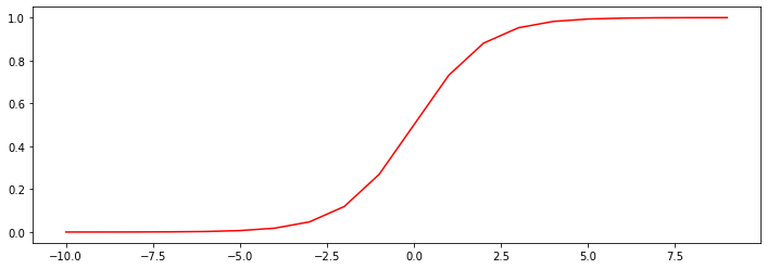
Sigmoid
- (g:mathbb{R} o [0,1])
- (g(0)=0.5)
- (g(- infty)=0)
- (g(+ infty)=1)
def model(X, theta):

    return sigmoid(np.dot(X, theta.T))
[egin{array}{ccc}
egin{pmatrix} heta_{0} & heta_{1} & heta_{2}end{pmatrix} & imes & egin{pmatrix}1\
x_{1}\
x_{2}
end{pmatrix}end{array}= heta_{0}+ heta_{1}x_{1}+ heta_{2}x_{2}
]
pdData.insert(0, 'Ones', 1) # in a try / except structure so as not to return an error if the block si executed several times


# set X (training data) and y (target variable)
orig_data = pdData.as_matrix() # convert the Pandas representation of the data to an array useful for further computations
cols = orig_data.shape[1]
X = orig_data[:,0:cols-1]
y = orig_data[:,cols-1:cols]

# convert to numpy arrays and initalize the parameter array theta
#X = np.matrix(X.values)
#y = np.matrix(data.iloc[:,3:4].values) #np.array(y.values)
theta = np.zeros([1, 3])
d:pythonpy376libsite-packagesipykernel_launcher.py:5: FutureWarning: Method .as_matrix will be removed in a future version. Use .values instead.
  """
X[:5]
array([[ 1.        , 34.62365962, 78.02469282],
       [ 1.        , 30.28671077, 43.89499752],
       [ 1.        , 35.84740877, 72.90219803],
       [ 1.        , 60.18259939, 86.3085521 ],
       [ 1.        , 79.03273605, 75.34437644]])
y[:5]
array([[0.],
       [0.],
       [0.],
       [1.],
       [1.]])
theta
array([[0., 0., 0.]])
X.shape, y.shape, theta.shape
((100, 3), (100, 1), (1, 3))
损失函数
将对数似然函数去负号
[D(h_ heta(x), y) = -ylog(h_ heta(x)) - (1-y)log(1-h_ heta(x))
]
求平均损失
[J( heta)=frac{1}{n}sum_{i=1}^{n} D(h_ heta(x_i), y_i)
]
def cost(X, y, theta):
    left = np.multiply(-y, np.log(model(X, theta)))
    right = np.multiply(1 - y, np.log(1 - model(X, theta)))
    return np.sum(left - right) / (len(X))
cost(X, y, theta)
0.6931471805599453
计算梯度
[frac{partial J}{partial heta_j}=-frac{1}{m}sum_{i=1}^n (y_i - h_ heta (x_i))x_{ij}
]
def gradient(X, y, theta):
    grad = np.zeros(theta.shape)
    error = (model(X, theta)- y).ravel()
    for j in range(len(theta.ravel())): #for each parmeter
        term = np.multiply(error, X[:,j])
        grad[0, j] = np.sum(term) / len(X)

    return grad
Gradient descent
比较3中不同梯度下降方法
STOP_ITER = 0
STOP_COST = 1
STOP_GRAD = 2

def stopCriterion(type, value, threshold):
    #设定三种不同的停止策略
    if type == STOP_ITER:        return value > threshold
    elif type == STOP_COST:      return abs(value[-1]-value[-2]) < threshold
    elif type == STOP_GRAD:      return np.linalg.norm(value) < threshold
import numpy.random
#洗牌
def shuffleData(data):
    np.random.shuffle(data)
    cols = data.shape[1]
    X = data[:, 0:cols-1]
    y = data[:, cols-1:]
    return X, y
import time

def descent(data, theta, batchSize, stopType, thresh, alpha):
    #梯度下降求解

    init_time = time.time()
    i = 0 # 迭代次数
    k = 0 # batch
    X, y = shuffleData(data)
    grad = np.zeros(theta.shape) # 计算的梯度
    costs = [cost(X, y, theta)] # 损失值


    while True:
        grad = gradient(X[k:k+batchSize], y[k:k+batchSize], theta)
        k += batchSize #取batch数量个数据
        if k >= n:
            k = 0
            X, y = shuffleData(data) #重新洗牌
        theta = theta - alpha*grad # 参数更新
        costs.append(cost(X, y, theta)) # 计算新的损失
        i += 1

        if stopType == STOP_ITER:       value = i
        elif stopType == STOP_COST:     value = costs
        elif stopType == STOP_GRAD:     value = grad
        if stopCriterion(stopType, value, thresh): break

    return theta, i-1, costs, grad, time.time() - init_time
def runExpe(data, theta, batchSize, stopType, thresh, alpha):
    #import pdb; pdb.set_trace();
    theta, iter, costs, grad, dur = descent(data, theta, batchSize, stopType, thresh, alpha)
    name = "Original" if (data[:,1]>2).sum() > 1 else "Scaled"
    name += " data - learning rate: {} - ".format(alpha)
    if batchSize==n: strDescType = "Gradient"
    elif batchSize==1:  strDescType = "Stochastic"
    else: strDescType = "Mini-batch ({})".format(batchSize)
    name += strDescType + " descent - Stop: "
    if stopType == STOP_ITER: strStop = "{} iterations".format(thresh)
    elif stopType == STOP_COST: strStop = "costs change < {}".format(thresh)
    else: strStop = "gradient norm < {}".format(thresh)
    name += strStop
    print ("***{}
Theta: {} - Iter: {} - Last cost: {:03.2f} - Duration: {:03.2f}s".format(
        name, theta, iter, costs[-1], dur))
    fig, ax = plt.subplots(figsize=(12,4))
    ax.plot(np.arange(len(costs)), costs, 'r')
    ax.set_xlabel('Iterations')
    ax.set_ylabel('Cost')
    ax.set_title(name.upper() + ' - Error vs. Iteration')
    return theta
不同的停止策略
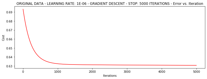
设定迭代次数
#选择的梯度下降方法是基于所有样本的
n=100
runExpe(orig_data, theta, n, STOP_ITER, thresh=5000, alpha=0.000001)
***Original data - learning rate: 1e-06 - Gradient descent - Stop: 5000 iterations
Theta: [[-0.00027127  0.00705232  0.00376711]] - Iter: 5000 - Last cost: 0.63 - Duration: 1.47s


array([[-0.00027127,  0.00705232,  0.00376711]])
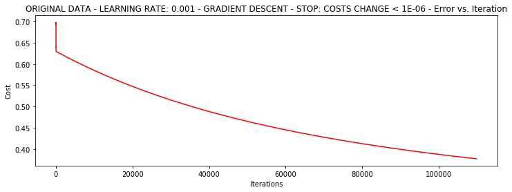
根据损失值停止
设定阈值 1E-6, 差不多需要110 000次迭代
runExpe(orig_data, theta, n, STOP_COST, thresh=0.000001, alpha=0.001)
***Original data - learning rate: 0.001 - Gradient descent - Stop: costs change < 1e-06
Theta: [[-5.13364014  0.04771429  0.04072397]] - Iter: 109901 - Last cost: 0.38 - Duration: 32.65s


array([[-5.13364014,  0.04771429,  0.04072397]])
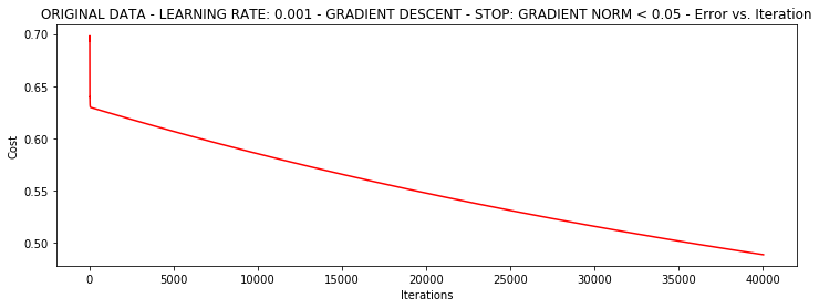
根据梯度变化停止
设定阈值 0.05,差不多需要40 000次迭代
runExpe(orig_data, theta, n, STOP_GRAD, thresh=0.05, alpha=0.001)
***Original data - learning rate: 0.001 - Gradient descent - Stop: gradient norm < 0.05
Theta: [[-2.37033409  0.02721692  0.01899456]] - Iter: 40045 - Last cost: 0.49 - Duration: 12.20s


array([[-2.37033409,  0.02721692,  0.01899456]])
对比不同的梯度下降方法
Stochastic descent
runExpe(orig_data, theta, 1, STOP_ITER, thresh=5000, alpha=0.001)
***Original data - learning rate: 0.001 - Stochastic descent - Stop: 5000 iterations
Theta: [[-0.36656341 -0.01406809 -0.01956622]] - Iter: 5000 - Last cost: 1.80 - Duration: 0.45s


array([[-0.36656341, -0.01406809, -0.01956622]])
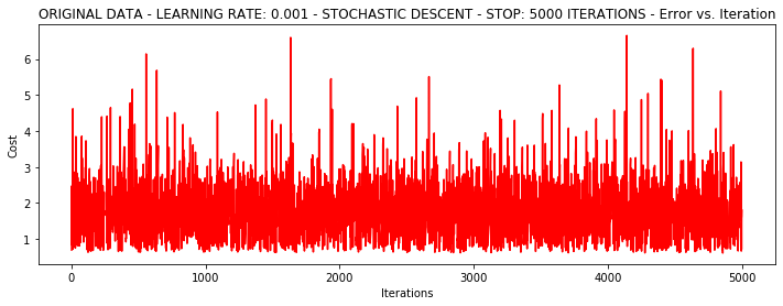
有点爆炸。。。很不稳定,再来试试把学习率调小一些
runExpe(orig_data, theta, 1, STOP_ITER, thresh=15000, alpha=0.000002)
***Original data - learning rate: 2e-06 - Stochastic descent - Stop: 15000 iterations
Theta: [[-0.00202316  0.00991808  0.00087764]] - Iter: 15000 - Last cost: 0.63 - Duration: 1.38s


array([[-0.00202316,  0.00991808,  0.00087764]])
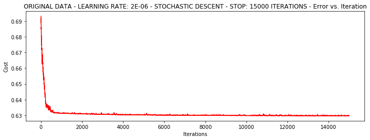
速度快,但稳定性差,需要很小的学习率
Mini-batch descent
runExpe(orig_data, theta, 16, STOP_ITER, thresh=15000, alpha=0.001)
***Original data - learning rate: 0.001 - Mini-batch (16) descent - Stop: 15000 iterations
Theta: [[-1.03398289  0.04372859  0.02318741]] - Iter: 15000 - Last cost: 1.05 - Duration: 1.83s


array([[-1.03398289,  0.04372859,  0.02318741]])
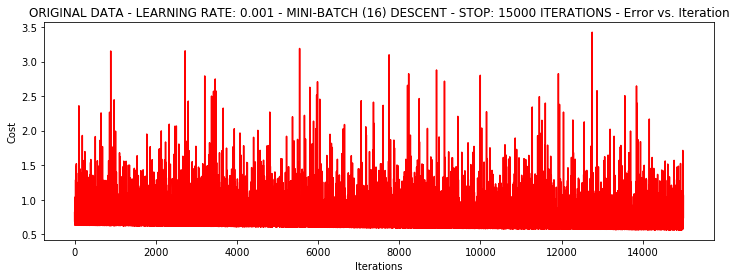
浮动仍然比较大,我们来尝试下对数据进行标准化
将数据按其属性(按列进行)减去其均值,然后除以其方差。最后得到的结果是,对每个属性/每列来说所有数据都聚集在0附近,方差值为1
from sklearn import preprocessing as pp

scaled_data = orig_data.copy()
scaled_data[:, 1:3] = pp.scale(orig_data[:, 1:3])

runExpe(scaled_data, theta, n, STOP_ITER, thresh=5000, alpha=0.001)
***Scaled data - learning rate: 0.001 - Gradient descent - Stop: 5000 iterations
Theta: [[0.3080807  0.86494967 0.77367651]] - Iter: 5000 - Last cost: 0.38 - Duration: 1.56s


array([[0.3080807 , 0.86494967, 0.77367651]])
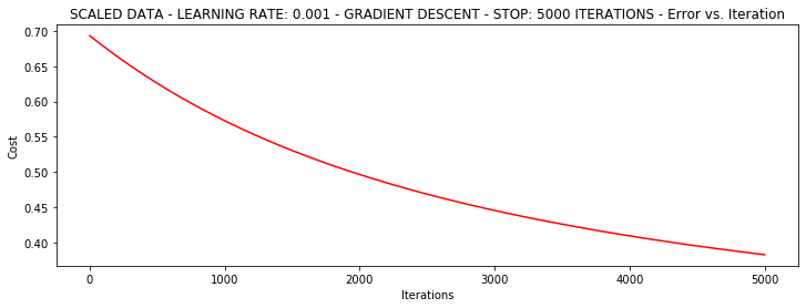
它好多了!原始数据,只能达到达到0.61,而我们得到了0.38个在这里!
所以对数据做预处理是非常重要的
runExpe(scaled_data, theta, n, STOP_GRAD, thresh=0.02, alpha=0.001)
***Scaled data - learning rate: 0.001 - Gradient descent - Stop: gradient norm < 0.02
Theta: [[1.0707921  2.63030842 2.41079787]] - Iter: 59422 - Last cost: 0.22 - Duration: 19.58s


array([[1.0707921 , 2.63030842, 2.41079787]])
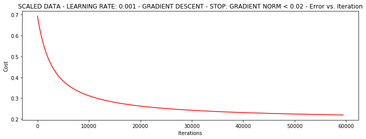
更多的迭代次数会使得损失下降的更多!
theta = runExpe(scaled_data, theta, 1, STOP_GRAD, thresh=0.002/5, alpha=0.001)
***Scaled data - learning rate: 0.001 - Stochastic descent - Stop: gradient norm < 0.0004
Theta: [[1.14964649 2.79191694 2.56889202]] - Iter: 72692 - Last cost: 0.22 - Duration: 8.55s
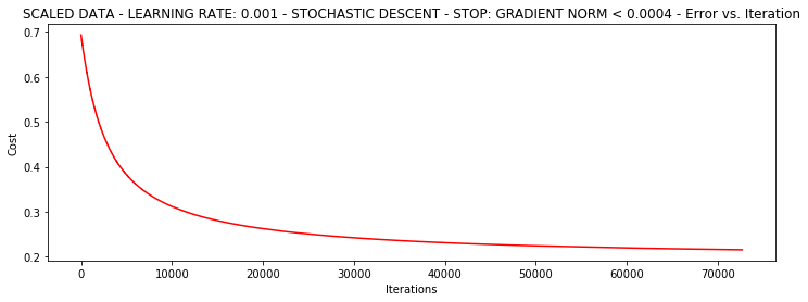
随机梯度下降更快,但是我们需要迭代的次数也需要更多,所以还是用batch的比较合适!!!
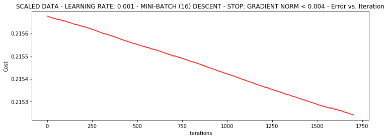
runExpe(scaled_data, theta, 16, STOP_GRAD, thresh=0.002*2, alpha=0.001)
***Scaled data - learning rate: 0.001 - Mini-batch (16) descent - Stop: gradient norm < 0.004
Theta: [[1.15785505 2.80909166 2.5880511 ]] - Iter: 1700 - Last cost: 0.22 - Duration: 0.36s


array([[1.15785505, 2.80909166, 2.5880511 ]])
精度
#设定阈值
def predict(X, theta):
    return [1 if x >= 0.5 else 0 for x in model(X, theta)]
scaled_X = scaled_data[:, :3]
y = scaled_data[:, 3]
predictions = predict(scaled_X, theta)
correct = [1 if ((a == 1 and b == 1) or (a == 0 and b == 0)) else 0 for (a, b) in zip(predictions, y)]
accuracy = (sum(map(int, correct)) % len(correct))
print ('accuracy = {0}%'.format(accuracy))
accuracy = 89%