sigmoid函数
g
(
z
)
=
1
1
+
e
−
z
g(z) = frac{1}{1+e^{-z}}
g(z)=1+e−z1
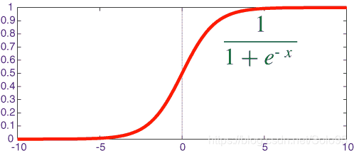
logistic使用sigmoid函数作为hypothesis,因为其值落于0和1之间,因此选定一个阀值就可以进行二元分类,这是机器学习的入门部分,理论不再赘述。
损失函数
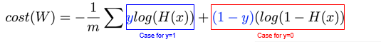
我们这里使用交叉熵(cross-entroy)来作为logistic regerssion的损失函数。
交叉熵计算公式为:
c
o
s
t
(
W
,
b
)
=
∑
i
=
1
m
y
l
o
g
(
h
(
x
)
)
cost(W,b)=sum_{i=1}^{m}ylog(h(x))
cost(W,b)=i=1∑mylog(h(x))
我们这里使用的交叉熵包含两部分是因为
y
=
1
y=1
y=1和
y
=
0
y=0
y=0两种情况对应了两个计算方法。
实现
tensorflow实现如下, 我给每一个部分加了详细且准确的注释:
import tensorflow as tf

# traing data
x_data = [[1, 2], [2, 3], [3, 1], [4, 3], [5, 3], [6, 2]]
y_data = [[0], [0], [0], [1], [1], [1]]

# placeholder for a tensor that will be fed at the traing phase
X = tf.placeholder(tf.float32, shape=[None, 2])
Y = tf.placeholder(tf.float32, shape=[None, 1])

# define hyperparameter
W = tf.Variable(tf.random_normal([2, 1]), name="weight")
b = tf.Variable(tf.random_normal([1]), name="bias")

# sigmoid hypothesis: tf.div(1., 1. + tf.exp(tf.matmul(X, W) + b))
hypothesis = tf.sigmoid(tf.matmul(X, W) + b)

# loss function: cross entropy loss function
cost = -tf.reduce_mean(Y * tf.log(hypothesis) + (1 - Y) * tf.log(1 - hypothesis))

train = tf.train.GradientDescentOptimizer(learning_rate=0.01).minimize(cost)

# if hypothesis > 0.5 1.(True) else 0.(False)
# therefore logistic regression is often used in binary classificaition
predicted = tf.cast(hypothesis > 0.5, dtype=tf.float32)

# compute accuracy
accuracy = tf.reduce_mean(tf.cast(tf.equal(predicted,Y), dtype=tf.float32))

# Start session
with tf.Session() as sess:
    # initialize global variable
    sess.run(tf.global_variables_initializer())

    for step in range(10001):
        cost_val, _ = sess.run([cost, train], feed_dict={X: x_data, Y: y_data})
        if step % 200 == 0:
            print(step, cost_val)

    # accuracy
    h, c, a = sess.run([hypothesis, predicted, accuracy], feed_dict={X: x_data, Y: y_data})
    print("
Hypothesis:
", h, "
Correct:
", c, "
Accuracy:
", a)
0 0.6799795
200 0.6385348
400 0.61319155
600 0.58977795
800 0.5677751
1000 0.5469113
1200 0.527039
1400 0.508074
1600 0.48996434
1800 0.47267392
2000 0.456174
2200 0.44043824
2400 0.4254409
2600 0.4111558
2800 0.39755583
3000 0.38461265
3200 0.3722982
3400 0.36058354
3600 0.34944
3800 0.33883914
4000 0.32875317
4200 0.31915486
4400 0.3100181
4600 0.3013176
4800 0.29302916
5000 0.28512976
5200 0.27759746
5400 0.27041152
5600 0.26355234
5800 0.25700125
6000 0.2507409
6200 0.24475472
6400 0.23902722
6600 0.233544
6800 0.2282914
7000 0.22325666
7200 0.21842766
7400 0.21379335
7600 0.20934318
7800 0.20506714
8000 0.20095605
8200 0.1970012
8400 0.19319443
8600 0.18952823
8800 0.1859952
9000 0.18258892
9200 0.17930289
9400 0.1761312
9600 0.17306834
9800 0.17010897
10000 0.16724814

Hypothesis:
 [[0.03854486]
 [0.16824016]
 [0.3402725 ]
 [0.76564145]
 [0.9292265 ]
 [0.97676086]]
Correct:
 [[0.]
 [0.]
 [0.]
 [1.]
 [1.]
 [1.]]
Accuracy:
 1.0
因为是个很简单的例子,损失函数一直在下降,准确度是1。