一、Precision - Recall 的平衡
1)基础理论
- 调整阈值的大小,可以调节精准率和召回率的比重;
- 阈值:threshold,分类边界值,score > threshold 时分类为 1,score < threshold 时分类为 0;
- 阈值增大,精准率提高,召回率降低;阈值减小,精准率降低,召回率提高;
- 精准率和召回率是相互牵制,互相矛盾的两个变量,不能同时增高;
- 逻辑回归的决策边界不一定非是
 ,也可以是任意的值,可根据业务而定:
 ,大于 threshold 时分类为 1,小于 threshold 时分类为 0;
 - 推广到其它算法,先计算出一个分数值 score ,再与 threshold 比较做分类判定;
2)举例说明精准率和召回率相互制约的关系(一)
- 计算结果 score > 0 时,分类结果为 ★;score < 0 时,分类结果为 ●;
- ★ 类型为所关注的事件;
-
情景1:threshold = 0
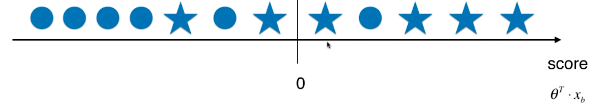
- 精准率:4 / 5 = 0.80;
- 召回率:4 / 6 = 0.67;
-
情景2:threshold > 0;
- 精准率:2 / 2 = 1.00;
- 召回率:2 / 6 = 0.33;
-
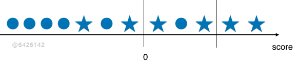
情景3:threshold < 0;

- 精准率:6 / 8 = 0.75;
- 召回率:6 / 6 = 1.00;
3)举例说明精准率和召回率相互制约的关系(二)
- LogisticRegression() 类中的 predict() 方法中,默认阈值 threshold 为 0,再根据 decision_function() 方法计算的待预测样本的 score 值进行对比分类:score < 0 分类结果为 0,score > 0 分类结果为 1;
- log_reg.decision_function(X_test):计算所有待预测样本的 score 值,以向量的数量类型返回结果;
- 此处的 score 值不是概率值,是另一种判断分类的方式中样本的得分,根据样本的得分对样本进行分类;
-
例
import numpy as np
from sklearn import datasets

digits = datasets.load_digits()
X = digits.data
y = digits.target.copy()
y[digits.target==9] = 1
y[digits.target!=9] = 0

from sklearn.model_selection import train_test_split
X_train, X_test, y_train, y_test = train_test_split(X, y, random_state=666)

from sklearn.linear_model import LogisticRegression
log_reg = LogisticRegression()
log_reg.fit(X_train, y_train)
-
阈值 threshold = 0
y_predict_1 = log_reg.predict(X_test)

from sklearn.metrics import confusion_matrix
confusion_matrix(y_test, y_predict_1)
# 混淆矩阵:array([[403, 2],
                  [9, 36]], dtype=int64)

from sklearn.metrics import precision_score
precision_score(y_test, y_predict_1)
# 精准率:0.9473684210526315

from sklearn.metrics import recall_score
recall_score(y_test, y_predict_1)
# 召回率:0.8
-
阈值 threshold = 5
decision_score = log_reg.decision_function(X_test)

# 更改 decision_score ,经过向量变化得到新的预测结果 y_predict_2;
# decision_score > 5,增大阈值为 5;(也就是提高判断标准)
y_predict_2 = np.array(decision_score >= 5, dtype='int')

confusion_matrix(y_test, y_predict_2)
# 混淆矩阵:array([[404,   1],
                 [ 21,  24]], dtype=int64)

precision_score(y_test, y_predict_2)
# 精准率:0.96

recall_score(y_test, y_predict_2)
# 召回率:0.5333333333333333
# 更改阈值的思路:基于 decision_function() 方法,改变 score 值,简介更阈值,不再经过 predict() 方法,而是经过向量变化得到新的分类结果;
-
阈值 threshold = -5
decision_score = log_reg.decision_function(X_test)
y_predict_3 = np.array(decision_score >= -5, dtype='int')

confusion_matrix(y_test, y_predict_3)
# 混淆矩阵:array([[390,  15],
                 [5,  40]], dtype=int64)

precision_score(y_test, y_predict_3)
# 精准率:0.7272727272727273

recall_score(y_test, y_predict_3)
# 召回率:0.8888888888888888
-
分析:
- 精准率和召回率相互牵制,相互平衡的,一个升高,另一个就会降低;
- 阈值越大,精准率越高,召回率越低;阈值越小,精准率越低,召回率越高;
- 更改阈值:1)通过 LogisticRegression() 模块下的 decision_function() 方法得到预测得分;2)不使用 predict() 方法,而是重新设定阈值,通过向量转化,直接根据预测得分进行样本分类;
二、精准率 - 召回率曲线(P - R 曲线)
- 对应分类算法,都可以调用其 decision_function() 方法,得到算法对每一个样本的决策的分数值;
- LogisticRegression() 算法中,默认的决策边界阈值为 0,样本的分数值大于 0,该样本分类为 1;样本的分数值小于 0,该样本分类为 0。
- 思路:随着阈值 threshold 的变化,精准率和召回率跟着相应变化;
- 设置不同的 threshold 值:
decision_scores = log_reg.decision_function(X_test)
thresholds = np.arange(np.min(decision_scores), np.max(decision_scores), 0.1)
# 0.1 是区间取值的步长;
1)编码实现 threshold - Precision、Recall 曲线和 P - R曲线
-
import numpy as np
import matplotlib.pyplot as plt
from sklearn import datasets

digits = datasets.load_digits()
X = digits.data
y = digits.target.copy()
y[digits.target==9] = 1
y[digits.target!=9] = 0

from sklearn.model_selection import train_test_split
X_train, X_test, y_train, y_test = train_test_split(X, y, random_state=666)

from sklearn.linear_model import LogisticRegression
log_reg = LogisticRegression()
log_reg.fit(X_train, y_train)
decision_scores = log_reg.decision_function(X_test)


from sklearn.metrics import precision_score
from sklearn.metrics import recall_score

precisions = []
recalls = []
thresholds = np.arange(np.min(decision_scores), np.max(decision_scores), 0.1)

for threshold in thresholds:
    y_predict = np.array(decision_scores >= threshold, dtype='int')
    precisions.append(precision_score(y_test, y_predict))
    recalls.append(recall_score(y_test, y_predict))
-
threshold - Precision、Recall 曲线
plt.plot(thresholds, precisions)
plt.plot(thresholds, recalls)
plt.show()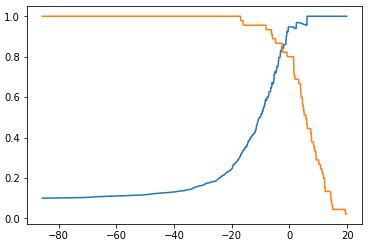
-
P - R 曲线
plt.plot(precisions, recalls)
plt.show()
2)scikit-learn 中 precision_recall_curve() 方法
- 根据 y_test、y_predicts 直接求解 precisions、recalls、thresholds;
from sklearn.metrics import precision_recall_curve
-
from sklearn.metrics import precision_recall_curve

precisions, recalls, thresholds = precision_recall_curve(y_test, decision_scores)

precisions.shape
# (145,)

recalls.shape
# (145,)

thresholds.shape
# (144,)
- 现象:thresholds 中的元素个数,比 precisions 和recalls 中的元素个数少 1 个;
- 原因:当 precision = 1、recall = 0 时,不存在 threshold;
-
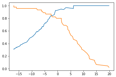
threshold - Precision、Recall 曲线
plt.plot(thresholds, precisions[:-1])
plt.plot(thresholds, recalls[:-1])
plt.show()
-
P - R 曲线
plt.plot(precisions, recalls)
plt.show()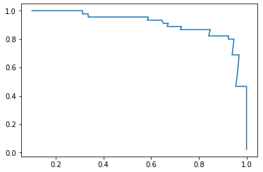
- 途中曲线开始急剧下降的点,可能就是精准率和召回率平衡位置的点;
3)分析
- 不同的模型对应的不同的 Precision - Recall 曲线:
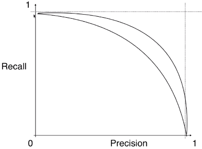
- 外层曲线对应的模型更优;或者称与坐标轴一起包围的面积越大者越优。
- P - R 曲线也可以作为选择算法、模型、超参数的指标;但一般不适用此曲线,而是使用 ROC 曲线;