对于平稳时间序列,可以建立趋势模型。当有理由相信这种趋势能够延伸到未来时,赋予变量t所需要的值,可以得到相应时刻的时间序列未来值,这就是趋势外推法
【分析实例】
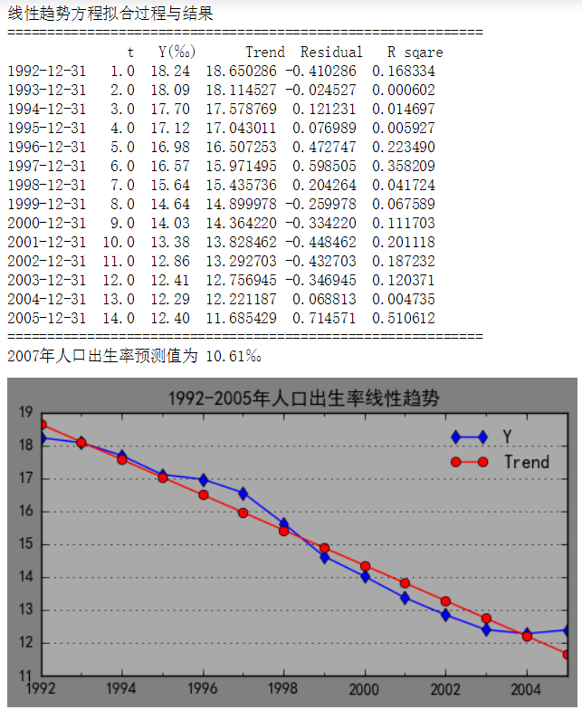
根据1992-2005年的人口出生率的数据,使用最小二乘法确定直线趋势方程,
1) 并计算各期的预测值和预测误差
2) 预测2007年的人口出生率


 1 import numpy as np
 2 import pandas as pd
 3 import matplotlib.pyplot as plt
 4
 5 def Line_Trend_Model( s, ):
 6     '''
 7     使用最小二乘法确定直线趋势方程
 8     输入值:s - pd.Series,index为连续型日期的Series
 9     返回值类型:字典
10     返回值:a - 截距,b - 斜率, sigma - 估计标准误差
11     '''
12     res = {}
13     n = len(s)
14     m = 2 # 用于计算估计标准误差,线性趋势方程对应的值为 2
15     res['t'] = [ i+1 for i in range(n)] #对t进行序号化处理
16     avg_t = np.mean(res['t'])
17     avg_y = np.mean(s)
18     ly = sum( map(lambda x,y:x * y, res['t'], s )) - n * avg_t * avg_y
19     lt = sum( map(lambda x:x**2, res['t'])) - n * avg_t ** 2
20     res['b'] = ly/lt #斜率
21     res['a'] = avg_y - res['b'] * avg_t # 截距
22     pre_y = res['a'] + res['b'] * np.array(res['t']) # 直线趋势线
23     res['sigma'] = np.sqrt(sum(map(lambda x,y:(x - y)**2, s, pre_y ))/(n-m)) # 估计的标准误差
24     return res
25
26 # 引入数据
27 data = [ 18.24, 18.09, 17.70, 17.12, 16.98, 16.57, 15.64, 14.64, 14.03, 13.38, 12.86, 12.41, 12.29, 12.40,]
28 dates = pd.date_range('1992-1-1', periods = len(data), freq = 'A') #'A'参数为每年的最后一天
29 y = pd.Series( data, index = dates )
30 # 计算值
31 param = Line_Trend_Model( y )
32 pre_y = param['a']+ param['b']* np.array(param['t']) # 趋势值
33 residual = y - pre_y #残差
34 db = pd.DataFrame( [ param['t'], data, list(pre_y), list(residual),  list(residual**2)],
35                     index = [ 't','Y(‰)','Trend','Residual','R sqare'],
36                     columns = dates ).T
37 # 输出结果
38 print('线性趋势方程拟合过程与结果')
39 print('='*60)
40 print(db)
41 print('='*60)
42 # 计算预测值
43 t = 16
44 yt = param['a']+ param['b']* t
45 print('2007年人口出生率预测值为 {:.2f}‰'.format(yt))
46 # 画图
47 fig = plt.figure( figsize = ( 6, 3 ), facecolor='grey' ) #设置画布背景色
48 ax=plt.subplot(111,axisbg = '#A9A9A9') # 设置子图背景色
49 db['Y(‰)'].plot( style = 'bd-',  label = 'Y' )
50 db['Trend'].plot( style = 'ro-', label = 'Trend')
51 legend = ax.legend(loc = 'best',frameon=False ) #云掉图例边框
52 #legend.get_frame().set_facecolor('#A9A9A9')#设置图例背景色
53 #legend.get_frame().set_edgecolor('#A9A9A9')#设置图例边框颜色
54 plt.grid( axis = 'y' )
55 plt.title('1992-2005年人口出生率线性趋势')
56
57 plt.show()
计算结果:
资料来源:刘春英《应用统计学》--中国金融出版社