一、MNIST实验内容
MNIST的实验比较简单,可以直接通过下面的程序加上程序上的部分注释就能很好的理解了,后面在完善具体的相关的数学理论知识,先记录在这里:
代码如下所示:
import tensorflow as tf
from tensorflow.examples.tutorials.mnist import input_data
import matplotlib.pyplot as plt
import numpy as np

%matplotlib inline

mnist = input_data.read_data_sets('/home/ubuntu-mm/TensorFlow/Learning/MNIST_data', one_hot=True) #下载MINIST数据集

#表示输入任意数量的MNIST图像,每一张图展平成784维的向量
#placeholder是占位符,在训练时指定
x = tf.placeholder(tf.float32, [None, 784])

#初始化W,b矩阵
W = tf.Variable(tf.zeros([784,10]))
b = tf.Variable(tf.zeros([10]))

#tf.matmul(X,W)表示x乘以W
y = tf.nn.softmax(tf.matmul(x, W) + b)

#为了计算交叉熵,我们首先需要添加一个新的占位符用于输入正确值
y_ = tf.placeholder("float", [None,10])

#交叉熵损失函数
cross_entropy = -tf.reduce_sum(y_*tf.log(y))

#模型的训练,不断的降低成本函数
#要求TensorFlow用梯度下降算法(gradient descent algorithm)以0.01的学习速率最小化交叉熵
train_step = tf.train.GradientDescentOptimizer(0.01).minimize(cross_entropy)

#在运行计算之前,需要添加一个操作来初始化我们创建的变量
init = tf.global_variables_initializer()

#在Session里面启动我模型,并且初始化变量
with tf.Session() as sess:
# sess = tf.Session()
# sess.run(init)
    sess.run(init)
    #开始训练模型,循环训练1000次
    for i in range(50):
        #随机抓取训练数据中的100个批处理数据点
      batch_xs, batch_ys = mnist.train.next_batch(100)
      #然后我们用这些数据点作为参数替换之前的占位符来运行train_step
      sess.run(train_step, feed_dict={x: batch_xs, y_: batch_ys})
    #检验真实标签与预测标签是否一致
    correct_prediction = tf.equal(tf.argmax(y,1), tf.argmax(y_,1))
    #计算精确度,将true和false转化成相应的浮点数,求和取平均
    accuracy = tf.reduce_mean(tf.cast(correct_prediction, "float"))
    #计算所学习到的模型在测试数据集上面的正确率
    print(sess.run(accuracy, feed_dict={x: mnist.test.images, y_: mnist.test.labels}))
    print 'W is:',W.eval()[10]
    print 'b is:',b.eval()
    batch_xs, batch_ys = mnist.train.next_batch(100)
#     print 'batch_xs[1]=',batch_xs[1]
    print 'batch_ys[1]=',batch_ys[1]
    x_in = tf.reshape(batch_xs[1],[1,784])
    Y_Predict = tf.nn.softmax(tf.matmul(x_in, W) + b)
    print 'Y_Predict is :',Y_Predict.eval()
Ori_Pic = np.zeros([28,28])
for m in range(784):
    i = m%28
    j = (m-i)/28
    Ori_Pic[j][i] = batch_xs[1][m]
plt.figure(1)
plt.imshow(Ori_Pic)
实验运行的结果如下所示:
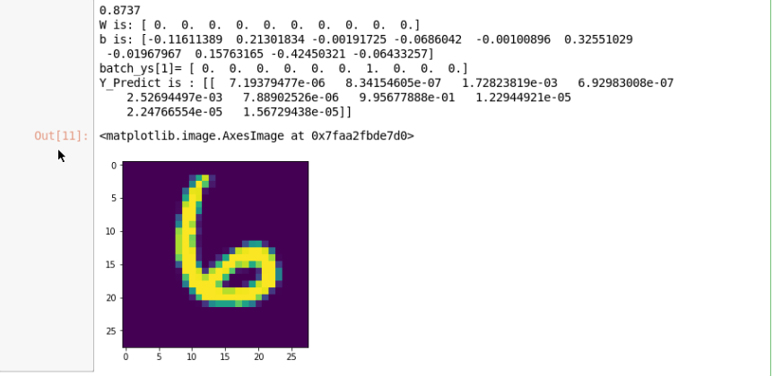 由结果显示的可知:图片对应为6的概率是99.56%
二、交叉熵损失函数的基本原理: