Aspheric Coefficients
| R | k | A4 | A6 | A8 | A10 | A12 | A14 | A16 | |
| S1 | PLANO | - | - | - | - | - | - | - | - |
| S2 | 2.68415 | -0.517612 | -5.980307E-5 | 1.527613E-5 | 3.647708E-6 | -1.381275E-7 | 4.485638E-8 | - | - |
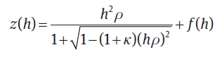
Aspheric Lens Equation
Aspheric Surface Structure
2. 2D Geometry Analysis
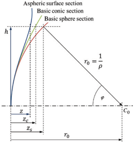
3. Equation

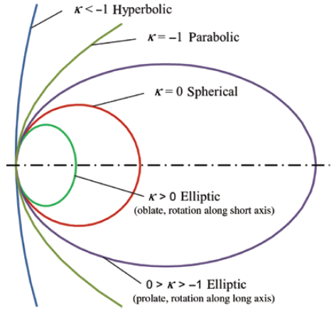
此处使用了非球面棱镜中最基本的面型之一(幂级数),对于非球面棱镜的球面方程,主要分为两个部分组成,前部分为基本的圆锥曲面部分,后部分一般为多项式部分(Polynomials-多项式方程: Power幂级数、Zernike多项式、Qcon多项式等), 基本形式如下所示:
- Power Series
- Zernike polynomials

- Qcon polynomials
- Q polynomials
对于上述各类型的多项式部分,其随着非球面高度位置的变化情况如下:


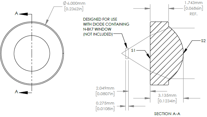
Basic Parameter of Lens
- MATERIAL: D-ZK3
- REFRACTIVE INDEX: 1.583 ±0.002
- DESIGN WAVELENGTH: 655 nm
- CLEAR APERTURE: (S1) 3.38 mm (S2) 4.80 mm
- EFFECTIVE FOCAL LENGTH: 4.6 mm±1%
- NUMERICAL APERTURE: 0.5
- DIAMETER TOLERANCE: ±0.015 mm
- CENTER THICKNESS TOLERANCE: ±0.020 mm
- SURFACE QUALITY: 40-20 SCRATCH-DIG (INCLUDES ENTIRE BULK MATERIAL)
- RMS WFE: ≤ DIFFRACTION LIMITED
- COATING(S1&S2): BBAR Ravg<0.5% FROM 350-700 nm, 0 AOI
Light Line Trace Simulation with MATLAB(基于MATLAB的光线追迹)
 1 clc;
 2 clear;
 3
 4 % Here the Aspheric function parameter.
 5 R = 2.684150;
 6 k = -0.517612;
 7 A4 = -5.980307E-5;
 8 A6 = 1.527613E-5;
 9 A8 = 3.647708E-6;
10 A10 = -1.381275E-7;
11 A12 = 4.485638E-8;
12
13 Lens_Aspheric_hRange = 5.1; % This the Aspheric h Range.
14
15 Slice = 100; % Data Slice number.
16
17 y = linspace(0,Lens_Aspheric_hRange/2,Slice); % h direction linspace data slice.
18 z=y.^2./R./(1+sqrt(1-(1+k)*y.^2./R^2)) + A4*y.^4 + A6*y.^6 + A8*y.^8 + A10*y.^10 +A12*y.^12; % Caculate the z direction axis value.
19 plot(y,z)
20 axis equal
21
22 syms Aspheric_Func(x)
23 Aspheric_Func(x) = x^2/R/(1+sqrt(1-(1+k)*x^2/R^2)) + A4*x^4 + A6*x^6 + A8*x^8 + A10*x^10 +A12*x^12; % Aspheric surface description function.
24 diff_Aspheric = diff(Aspheric_Func,x); % The Slope function of the Aspheric surface description function.
25 plot(y,Aspheric_Func(y))
26 hold on
27
28 Lens_Square_thickness = 1.743; % Square Zone thickness value.
29 Lens_thickness = 3.135; % Totally Lens thickness value.
30 Lens_Aspheric_thickness = Lens_thickness - Lens_Square_thickness; % Aspheric zone thickness.
31 max(double(Aspheric_Func(y)));
32
33 syms PLANO_Func(x)
34 PLANO_Func(x) = Lens_thickness; % First Seperate
35 plot(y,PLANO_Func(y))
36 light_O = [0,4.41]; % 5.41 is the Focus position
37 plot(light_O(1),light_O(2),'*') % Plot the Laser Light Point O.
38
39 light_line_S1_K = (light_O(2) - PLANO_Func(y))./(light_O(1) - y); % Draw the Laser Light line from Point to PLANO.
40 Line_YRange = linspace(light_O(2),Lens_thickness,Slice); % The YRange data slice.
41 Line_Step = 5; % Set the Light Line simulation number.
42 syms x
43 for i=1:Line_Step:Slice
44     Line_XRange = (Line_YRange - light_O(2)) / light_line_S1_K(i); % Calculate the XRange data.
45     % fprintf('%d
',i)
46     plot(Line_XRange,Line_YRange) % Draw the Light line.
47 end
48 % axis equal
49 Light_iU = pi/2 - abs(double(atan(light_line_S1_K))); % Calculate the First input light theta angle.
50 n1 = 1.0; % The Refractive index of the Air.
51 n2 = 1.583; % The Refractive index of the Lens with the material D-ZK3.
52 theta_out = asin(sin(Light_iU)*n1./n2); % Caculate the First output
53 light_line_S2_K = -cot(theta_out); % Caculate the Slope of the Output Light Line.
54
55 cross_Point = zeros(2,Slice); % Create the Aspheric and Line Cross-Point Buff array.
56 syms Light_S2_Func(x)
57 for i=1:Line_Step:Slice
58     x_s = (Lens_thickness - light_O(2)) / light_line_S1_K(i); % Calculate the Start Point of the Light on PLANO.
59     Light_S2_Func(x) = (light_line_S2_K(i)*(x-x_s) + Lens_thickness); % Define the Light Line Func.
60     for xt = x_s:0.01:(x_s-Lens_thickness/light_line_S2_K(i)+0.02)
61         % temp = abs(Aspheric_Func(xt) - Light_S2_Func(xt))
62         if abs(Aspheric_Func(xt) - Light_S2_Func(xt)) < 0.1 % Calculate the Cross-Point Value.
63             cross_Point(:,i) = [xt,Aspheric_Func(xt)];
64             x_r = linspace(x_s,xt,100);
65             plot(x_r,Light_S2_Func(x_r)) % Draw the Light-Line Graph.
66             break
67         end
68     end
69 end
70
71 light_line_S3_K_Reg = zeros(1,Slice); % Alloc a Buffer for Storage the Slope of the Output Light Line.
72
73 for i=1:Line_Step:Slice
74     slope = diff_Aspheric(cross_Point(1,i)); % Calculate the Slope of the Aspheric surface.
75     % normal_alpha = atan(slope)+pi/2; % 法线角度(Units:rad)
76     Light_iU_S2 = atan(slope) - theta_out(i); % Calculate the input angle on the Aspheric surface.
77     Light_oU_S2 = asin(sin(Light_iU_S2)*n2./n1); % Calculate the output angle of the Aspheric surface.
78     light_line_S3_K_Reg(1,i) = tan(pi/2 - abs(Light_oU_S2) + atan(slope)); % Generate the Output Light line function.
79     y_res = linspace(cross_Point(2,i),-10);
80     x_res = (y_res - cross_Point(2,i)) / light_line_S3_K_Reg(1,i) + cross_Point(1,i);
81     plot(x_res,y_res) % Draw the Output Light Line.
82 end
83 axis equal
84 % plot(y,diff_Aspheric(y))
仿真追迹的结果如下:
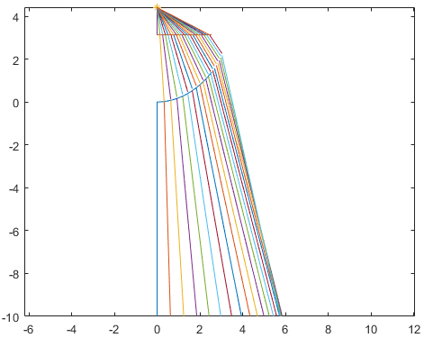
如果需要仿真不同位置点光源的发散汇聚的情况,只需要修改 `light_O = [0,4.41];` 部分即可调整Laser激光的出射位置,从而对光线进行追迹仿真,需要升入考虑的是光线在透镜中时,与非球面部分的交点计算采用了数值点代入验算的方式,效率较低,后期还需要对该方程的零解进行分析求解。
注:
1. 从上述仿真结果可以看出,当光线在非球面棱镜的边缘位置时,光线追迹的结果法线出射光线明显与其他部分的光线有交叠,因此非球面棱镜有一定的工作范围,需要严格注意。
2. 一定需要注意的是,在推导非球面棱镜的曲面方程时,需要注意不是圆锥曲线的方程推导,而是专属的非球面曲线构成的。
3. 对于非对称的非球面方程以及平移不变方程等特殊的方程类型,请参考《Description_of_aspheric_surfaces》