df = pd.read_csv("F:\kaggleDataSet\chennai-water\chennai_reservoir_levels.csv")
df["Date"] = pd.to_datetime(df["Date"], format='%d-%m-%Y')
df.head()

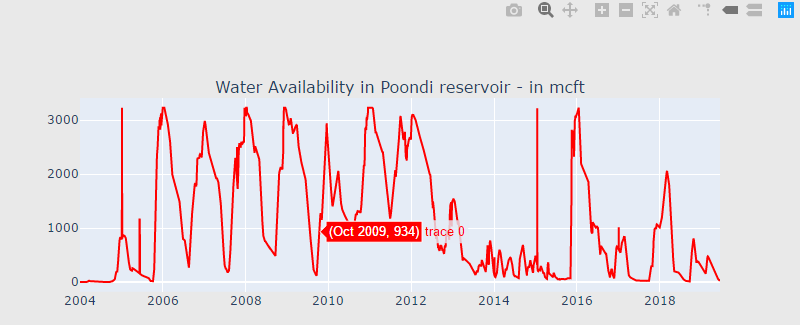
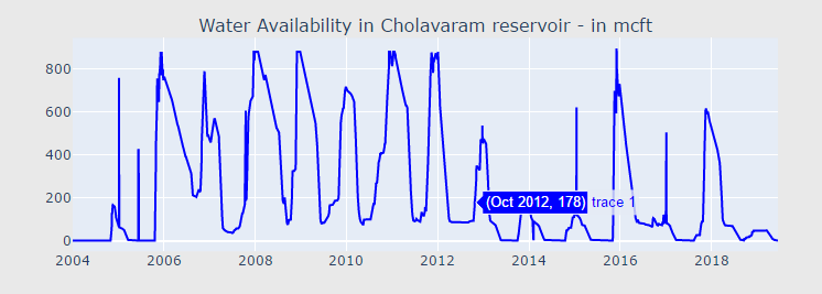
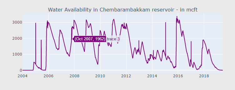
import datetime

def scatter_plot(cnt_srs, color):
    trace = go.Scatter(
        x=cnt_srs.index[::-1],
        y=cnt_srs.values[::-1],
        showlegend=False,
        marker=dict(
            color=color,
        ),
    )
    return trace

cnt_srs = df["POONDI"]
cnt_srs.index = df["Date"]
trace1 = scatter_plot(cnt_srs, 'red')

cnt_srs = df["CHOLAVARAM"]
cnt_srs.index = df["Date"]
trace2 = scatter_plot(cnt_srs, 'blue')

cnt_srs = df["REDHILLS"]
cnt_srs.index = df["Date"]
trace3 = scatter_plot(cnt_srs, 'green')

cnt_srs = df["CHEMBARAMBAKKAM"]
cnt_srs.index = df["Date"]
trace4 = scatter_plot(cnt_srs, 'purple')

subtitles = ["Water Availability in Poondi reservoir - in mcft",
             "Water Availability in Cholavaram reservoir - in mcft",
             "Water Availability in Redhills reservoir - in mcft",
             "Water Availability in Chembarambakkam reservoir - in mcft"
            ]
fig = tools.make_subplots(rows=4, cols=1, vertical_spacing=0.08,
                          subplot_titles=subtitles)
fig.append_trace(trace1, 1, 1)
fig.append_trace(trace2, 2, 1)
fig.append_trace(trace3, 3, 1)
fig.append_trace(trace4, 4, 1)
fig['layout'].update(height=1200, width=800, paper_bgcolor='rgb(233,233,233)')
py.iplot(fig, filename='h2o-plots')

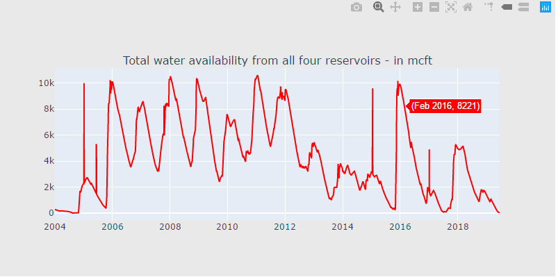
df["total"] = df["POONDI"] + df["CHOLAVARAM"] + df["REDHILLS"] + df["CHEMBARAMBAKKAM"]
df["total"] = df["POONDI"] + df["CHOLAVARAM"] + df["REDHILLS"] + df["CHEMBARAMBAKKAM"]

cnt_srs = df["total"]
cnt_srs.index = df["Date"]
trace5 = scatter_plot(cnt_srs, 'red')

fig = tools.make_subplots(rows=1, cols=1, vertical_spacing=0.08,
                          subplot_titles=["Total water availability from all four reservoirs - in mcft"])
fig.append_trace(trace5, 1, 1)


fig['layout'].update(height=400, width=800, paper_bgcolor='rgb(233,233,233)')
py.iplot(fig, filename='h2o-plots')
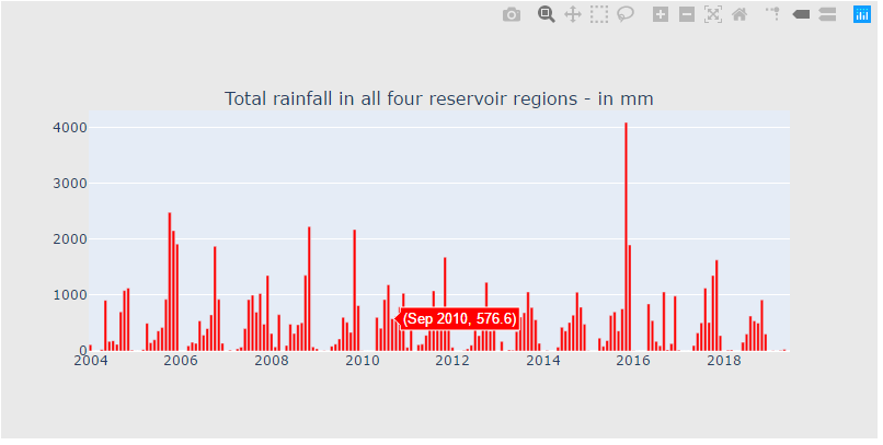
rain_df = pd.read_csv("F:\kaggleDataSet\chennai-water\chennai_reservoir_rainfall.csv")
rain_df["Date"] = pd.to_datetime(rain_df["Date"], format='%d-%m-%Y')

rain_df["total"] = rain_df["POONDI"] + rain_df["CHOLAVARAM"] + rain_df["REDHILLS"] + rain_df["CHEMBARAMBAKKAM"]
rain_df["total"] = rain_df["POONDI"] + rain_df["CHOLAVARAM"] + rain_df["REDHILLS"] + rain_df["CHEMBARAMBAKKAM"]

def bar_plot(cnt_srs, color):
    trace = go.Bar(
        x=cnt_srs.index[::-1],
        y=cnt_srs.values[::-1],
        showlegend=False,
        marker=dict(
            color=color,
        ))
    return trace

rain_df["YearMonth"] = pd.to_datetime(rain_df["Date"].dt.year.astype(str) + rain_df["Date"].dt.month.astype(str), format='%Y%m')

cnt_srs = rain_df.groupby("YearMonth")["total"].sum()
trace5 = bar_plot(cnt_srs, 'red')

fig = tools.make_subplots(rows=1, cols=1, vertical_spacing=0.08,
                          subplot_titles=["Total rainfall in all four reservoir regions - in mm"])
fig.append_trace(trace5, 1, 1)


fig['layout'].update(height=400, width=800, paper_bgcolor='rgb(233,233,233)')
py.iplot(fig, filename='h2o-plots')
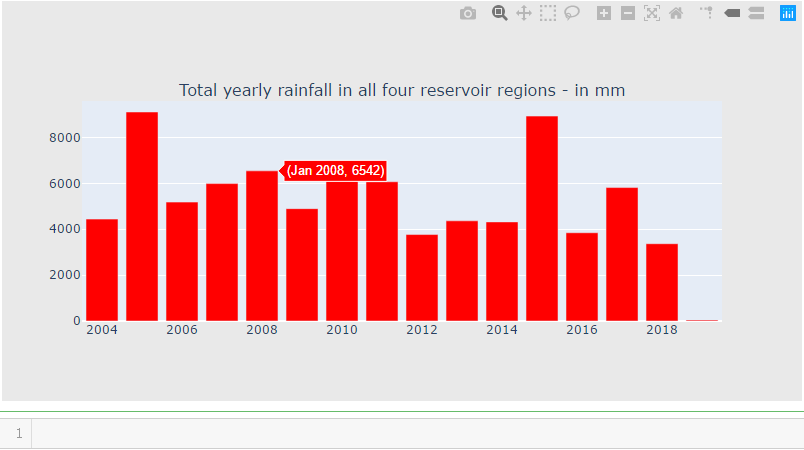
rain_df["Year"] = pd.to_datetime(rain_df["Date"].dt.year.astype(str), format='%Y')

cnt_srs = rain_df.groupby("Year")["total"].sum()
trace5 = bar_plot(cnt_srs, 'red')

fig = tools.make_subplots(rows=1, cols=1, vertical_spacing=0.08,
                          subplot_titles=["Total yearly rainfall in all four reservoir regions - in mm"])
fig.append_trace(trace5, 1, 1)


fig['layout'].update(height=400, width=800, paper_bgcolor='rgb(233,233,233)')
py.iplot(fig, filename='h2o-plots')
temp_df = df[(df["Date"].dt.month==2) & (df["Date"].dt.day==1)]

cnt_srs = temp_df["total"]
cnt_srs.index = temp_df["Date"]
trace5 = bar_plot(cnt_srs, 'red')

fig = tools.make_subplots(rows=1, cols=1, vertical_spacing=0.08,
                          subplot_titles=["Availability of total reservoir water (4 major ones) at the beginning of summer"])
fig.append_trace(trace5, 1, 1)


fig['layout'].update(height=400, width=800, paper_bgcolor='rgb(233,233,233)')
py.iplot(fig, filename='h2o-plots')

结论:
2004年的水资源短缺使维拉南湖成为城市供水的新途径。
希望目前的缺水能为这个陷入困境的城市带来更多额外的水源。在过去的15年里,这个城市发展了很多,因此需要额外的水资源来满足需求。
城市需要通过提前估计需求来设计更好的稀缺控制方法。现在,
“只有下雨才能拯救这座城市!”