


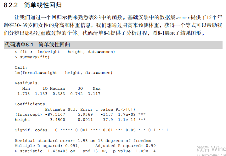

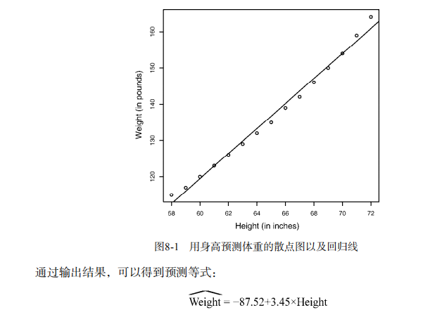

#------------------------------------------------------------#
# R in Action (2nd ed): Chapter 8                            #
# Regression                                                 #
# requires packages car, gvlma, MASS, leaps to be installed  #
# install.packages(c("car", "gvlma", "MASS", "leaps"))       #
#------------------------------------------------------------#

par(ask=TRUE)
opar <- par(no.readonly=TRUE)

# Listing 8.1 - Simple linear regression
fit <- lm(weight ~ height, data=women)
summary(fit)
women$weight
fitted(fit)
residuals(fit)
plot(women$height,women$weight,
     main="Women Age 30-39",
     xlab="Height (in inches)",
     ylab="Weight (in pounds)")
# add the line of best fit
abline(fit)


# Listing 8.2 - Polynomial regression
fit2 <- lm(weight ~ height + I(height^2), data=women)
summary(fit2)
plot(women$height,women$weight,
     main="Women Age 30-39",
     xlab="Height (in inches)",
     ylab="Weight (in lbs)")
lines(women$height,fitted(fit2))


# Enhanced scatterplot for women data
library(car)
library(car)
scatterplot(weight ~ height, data=women,
            spread=FALSE, smoother.args=list(lty=2), pch=19,
            main="Women Age 30-39",
            xlab="Height (inches)",
            ylab="Weight (lbs.)")


# Listing 8.3 - Examining bivariate relationships
states <- as.data.frame(state.x77[,c("Murder", "Population",
                                     "Illiteracy", "Income", "Frost")])
cor(states)
library(car)
scatterplotMatrix(states, spread=FALSE, smoother.args=list(lty=2),
                  main="Scatter Plot Matrix")


# Listing 8.4 - Multiple linear regression
states <- as.data.frame(state.x77[,c("Murder", "Population",
                                     "Illiteracy", "Income", "Frost")])
fit <- lm(Murder ~ Population + Illiteracy + Income + Frost, data=states)
summary(fit)


# Listing 8.5 - Mutiple linear regression with a significant interaction term
fit <- lm(mpg ~ hp + wt + hp:wt, data=mtcars)
summary(fit)

library(effects)
plot(effect("hp:wt", fit,, list(wt=c(2.2, 3.2, 4.2))), multiline=TRUE)

# simple regression diagnostics
fit <- lm(weight ~ height, data=women)
par(mfrow=c(2,2))
plot(fit)
newfit <- lm(weight ~ height + I(height^2), data=women)
par(opar)
par(mfrow=c(2,2))
plot(newfit)
par(opar)


# basic regression diagnostics for states data
opar <- par(no.readonly=TRUE)
fit <- lm(weight ~ height, data=women)
par(mfrow=c(2,2))
plot(fit)
par(opar)

fit2 <- lm(weight ~ height + I(height^2), data=women)
opar <- par(no.readonly=TRUE)
par(mfrow=c(2,2))
plot(fit2)
par(opar)


# Assessing normality
library(car)
states <- as.data.frame(state.x77[,c("Murder", "Population",
                                     "Illiteracy", "Income", "Frost")])
fit <- lm(Murder ~ Population + Illiteracy + Income + Frost, data=states)
qqPlot(fit, labels=row.names(states), id.method="identify",
       simulate=TRUE, main="Q-Q Plot")


# Listing 8.6 - Function for plotting studentized residuals
residplot <- function(fit, nbreaks=10) {
  z <- rstudent(fit)
  hist(z, breaks=nbreaks, freq=FALSE,
       xlab="Studentized Residual",
       main="Distribution of Errors")
  rug(jitter(z), col="brown")
  curve(dnorm(x, mean=mean(z), sd=sd(z)),
        add=TRUE, col="blue", lwd=2)
  lines(density(z)$x, density(z)$y,
        col="red", lwd=2, lty=2)
  legend("topright",
         legend = c( "Normal Curve", "Kernel Density Curve"),
         lty=1:2, col=c("blue","red"), cex=.7)
}

residplot(fit)


# Assessing linearity
library(car)
crPlots(fit)


# Listing 8.7 - Assessing homoscedasticity
library(car)
ncvTest(fit)
spreadLevelPlot(fit)


# Listing 8.8 - Global test of linear model assumptions
library(gvlma)
gvmodel <- gvlma(fit)
summary(gvmodel)

# Listing 8.9 - Evaluating multi-collinearity
library(car)
vif(fit)
sqrt(vif(fit)) > 2 # problem?

# Assessing outliers
library(car)
outlierTest(fit)

#  Identifying high leverage points
hat.plot <- function(fit) {
  p <- length(coefficients(fit))
  n <- length(fitted(fit))
  plot(hatvalues(fit), main="Index Plot of Hat Values")
  abline(h=c(2,3)*p/n, col="red", lty=2)
  identify(1:n, hatvalues(fit), names(hatvalues(fit)))
}
hat.plot(fit)

# Identifying influential observations

# Cooks Distance D
# identify D values > 4/(n-k-1)
cutoff <- 4/(nrow(states)-length(fit$coefficients)-2)
plot(fit, which=4, cook.levels=cutoff)
abline(h=cutoff, lty=2, col="red")

# Added variable plots
# add id.method="identify" to interactively identify points
library(car)
avPlots(fit, ask=FALSE, id.method="identify")

# Influence Plot
library(car)
influencePlot(fit, id.method="identify", main="Influence Plot",
              sub="Circle size is proportial to Cook's Distance" )


# Listing 8.10 - Box-Cox Transformation to normality
library(car)
summary(powerTransform(states$Murder))

# Box-Tidwell Transformations to linearity
library(car)
boxTidwell(Murder~Population+Illiteracy,data=states)


# Listing 8.11 - Comparing nested models using the anova function
states <- as.data.frame(state.x77[,c("Murder", "Population",
                                     "Illiteracy", "Income", "Frost")])
fit1 <- lm(Murder ~ Population + Illiteracy + Income + Frost,
           data=states)
fit2 <- lm(Murder ~ Population + Illiteracy, data=states)
anova(fit2, fit1)


# Listing 8.12 - Comparing models with the AIC
fit1 <- lm(Murder ~ Population + Illiteracy + Income + Frost,
           data=states)
fit2 <- lm(Murder ~ Population + Illiteracy, data=states)
AIC(fit1,fit2)


# Listing 8.13 - Backward stepwise selection
library(MASS)
states <- as.data.frame(state.x77[,c("Murder", "Population",
                                     "Illiteracy", "Income", "Frost")])
fit <- lm(Murder ~ Population + Illiteracy + Income + Frost,
          data=states)
stepAIC(fit, direction="backward")


# Listing 8.14 - All subsets regression
library(leaps)
states <- as.data.frame(state.x77[,c("Murder", "Population",
                                     "Illiteracy", "Income", "Frost")])
leaps <-regsubsets(Murder ~ Population + Illiteracy + Income +
                     Frost, data=states, nbest=4)
plot(leaps, scale="adjr2")
library(car)
subsets(leaps, statistic="cp",
        main="Cp Plot for All Subsets Regression")
abline(1,1,lty=2,col="red")


# Listing 8.15 - Function for k-fold cross-validated R-square
shrinkage <- function(fit,k=10){
  require(bootstrap)

  # define functions
  theta.fit <- function(x,y){lsfit(x,y)}
  theta.predict <- function(fit,x){cbind(1,x)%*%fit$coef}

  # matrix of predictors
  x <- fit$model[,2:ncol(fit$model)]
  # vector of predicted values
  y <- fit$model[,1]

  results <- crossval(x,y,theta.fit,theta.predict,ngroup=k)
  r2 <- cor(y, fit$fitted.values)**2 # raw R2
  r2cv <- cor(y,results$cv.fit)**2 # cross-validated R2
  cat("Original R-square =", r2, "
")
  cat(k, "Fold Cross-Validated R-square =", r2cv, "
")
  cat("Change =", r2-r2cv, "
")
}

# using it
states <- as.data.frame(state.x77[,c("Murder", "Population",
                                     "Illiteracy", "Income", "Frost")])
fit <- lm(Murder ~ Population + Income + Illiteracy + Frost, data=states)
shrinkage(fit)
fit2 <- lm(Murder~Population+Illiteracy,data=states)
shrinkage(fit2)

#  Calculating standardized regression coefficients
states <- as.data.frame(state.x77[,c("Murder", "Population",
                                     "Illiteracy", "Income", "Frost")])
zstates <- as.data.frame(scale(states))
zfit <- lm(Murder~Population + Income + Illiteracy + Frost, data=zstates)
coef(zfit)

# Listing 8.16 rlweights function for clculating relative importance of predictors
relweights <- function(fit,...){
  R <- cor(fit$model)
  nvar <- ncol(R)
  rxx <- R[2:nvar, 2:nvar]
  rxy <- R[2:nvar, 1]
  svd <- eigen(rxx)
  evec <- svd$vectors
  ev <- svd$values
  delta <- diag(sqrt(ev))
  lambda <- evec %*% delta %*% t(evec)
  lambdasq <- lambda ^ 2
  beta <- solve(lambda) %*% rxy
  rsquare <- colSums(beta ^ 2)
  rawwgt <- lambdasq %*% beta ^ 2
  import <- (rawwgt / rsquare) * 100
  import <- as.data.frame(import)
  row.names(import) <- names(fit$model[2:nvar])
  names(import) <- "Weights"
  import <- import[order(import),1, drop=FALSE]
  dotchart(import$Weights, labels=row.names(import),
           xlab="% of R-Square", pch=19,
           main="Relative Importance of Predictor Variables",
           sub=paste("Total R-Square=", round(rsquare, digits=3)),
           ...)
  return(import)
  }

  # Listing 8.17 - Applying the relweights function
  states <- as.data.frame(state.x77[,c("Murder", "Population",
                                       "Illiteracy", "Income", "Frost")])
  fit <- lm(Murder ~ Population + Illiteracy + Income + Frost, data=states)
  relweights(fit, col="blue")