


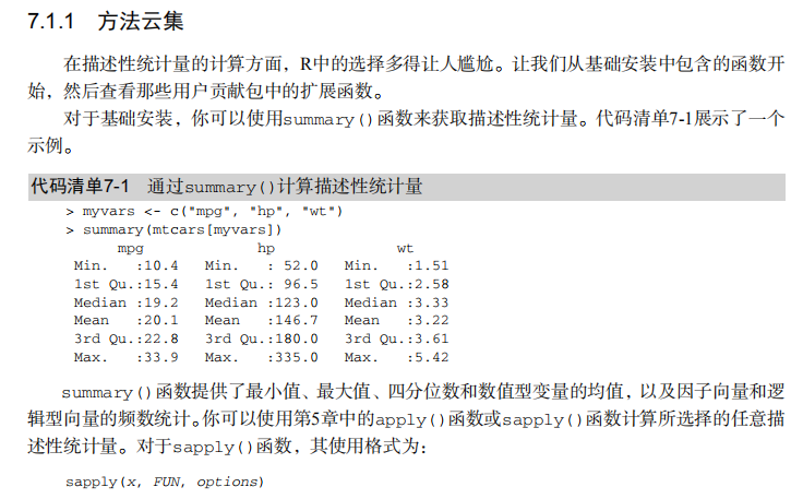

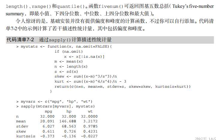


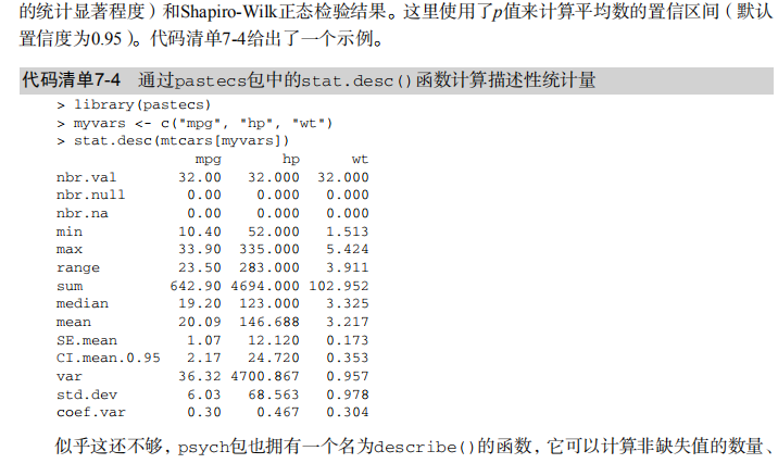
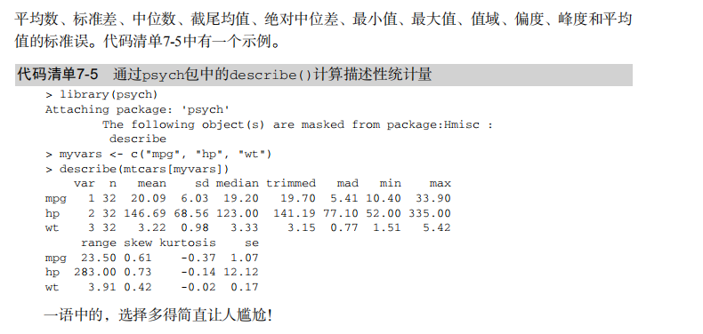


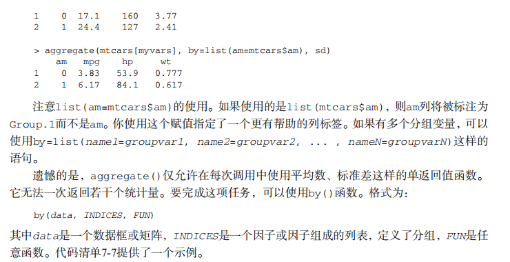
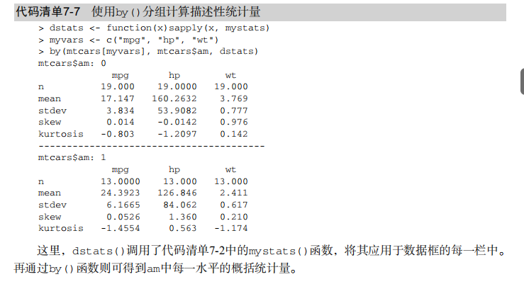
#---------------------------------------------------------------------#
# R in Action (2nd ed): Chapter 7                                     #
# Basic statistics                                                    #
# requires packages npmc, ggm, gmodels, vcd, Hmisc,                   #
#                   pastecs, psych, doBy to be installed              #
# install.packages(c("ggm", "gmodels", "vcd", "Hmisc",                #
#                    "pastecs", "psych", "doBy"))                     #
#---------------------------------------------------------------------#


mt <- mtcars[c("mpg", "hp", "wt", "am")]
head(mt)

# Listing 7.1 - Descriptive stats via summary
mt <- mtcars[c("mpg", "hp", "wt", "am")]
summary(mt)


# Listing 7.2 - descriptive stats via sapply
mystats <- function(x, na.omit=FALSE){
  if (na.omit)
    x <- x[!is.na(x)]
  m <- mean(x)
  n <- length(x)
  s <- sd(x)
  skew <- sum((x-m)^3/s^3)/n
  kurt <- sum((x-m)^4/s^4)/n - 3
  return(c(n=n, mean=m, stdev=s, skew=skew, kurtosis=kurt))
}

myvars <- c("mpg", "hp", "wt")
sapply(mtcars[myvars], mystats)


# Listing 7.3 - Descriptive stats via describe (Hmisc)
library(Hmisc)
myvars <- c("mpg", "hp", "wt")
describe(mtcars[myvars])


# Listing 7.,4 - Descriptive stats via stat.desc (pastecs)
library(pastecs)
myvars <- c("mpg", "hp", "wt")
stat.desc(mtcars[myvars])


# Listing 7.5 - Descriptive stats via describe (psych)
library(psych)
myvars <- c("mpg", "hp", "wt")
describe(mtcars[myvars])


# Listing 7.6 - Descriptive stats by group with aggregate
myvars <- c("mpg", "hp", "wt")
aggregate(mtcars[myvars], by=list(am=mtcars$am), mean)
aggregate(mtcars[myvars], by=list(am=mtcars$am), sd)


# Listing 7.7 - Descriptive stats by group via by
dstats <- function(x)sapply(x, mystats)
myvars <- c("mpg", "hp", "wt")
by(mtcars[myvars], mtcars$am, dstats)


# Listing 7.8 - Descriptive stats by group via summaryBy
library(doBy)
summaryBy(mpg+hp+wt~am, data=mtcars, FUN=mystats)


# Listing 7.9 - Descriptive stats by group via describe.by (psych)
library(psych)
myvars <- c("mpg", "hp", "wt")
describeBy(mtcars[myvars], list(am=mtcars$am))


# summary statistics by group via the reshape package
library(reshape)
dstats <- function(x)(c(n=length(x), mean=mean(x), sd=sd(x)))
dfm <- melt(mtcars, measure.vars=c("mpg", "hp", "wt"),
            id.vars=c("am", "cyl"))
cast(dfm, am + cyl + variable ~ ., dstats)


# frequency tables
library(vcd)
head(Arthritis)

# one way table
mytable <- with(Arthritis, table(Improved))
mytable  # frequencies
prop.table(mytable) # proportions
prop.table(mytable)*100 # percentages


# two way table
mytable <- xtabs(~ Treatment+Improved, data=Arthritis)
mytable # frequencies
margin.table(mytable,1) #row sums
margin.table(mytable, 2) # column sums
prop.table(mytable) # cell proportions
prop.table(mytable, 1) # row proportions
prop.table(mytable, 2) # column proportions
addmargins(mytable) # add row and column sums to table

# more complex tables
addmargins(prop.table(mytable))
addmargins(prop.table(mytable, 1), 2)
addmargins(prop.table(mytable, 2), 1)


# Listing 7.10 - Two way table using CrossTable
library(gmodels)
CrossTable(Arthritis$Treatment, Arthritis$Improved)


# Listing 7.11 - Three way table
mytable <- xtabs(~ Treatment+Sex+Improved, data=Arthritis)
mytable
ftable(mytable)
margin.table(mytable, 1)
margin.table(mytable, 2)
margin.table(mytable, 2)
margin.table(mytable, c(1,3))
ftable(prop.table(mytable, c(1,2)))
ftable(addmargins(prop.table(mytable, c(1, 2)), 3))

# Listing 7.12 - Chi-square test of independence
library(vcd)
mytable <- xtabs(~Treatment+Improved, data=Arthritis)
chisq.test(mytable)
mytable <- xtabs(~Improved+Sex, data=Arthritis)
chisq.test(mytable)


# Fisher's exact test
mytable <- xtabs(~Treatment+Improved, data=Arthritis)
fisher.test(mytable)


# Chochran-Mantel-Haenszel test
mytable <- xtabs(~Treatment+Improved+Sex, data=Arthritis)
mantelhaen.test(mytable)


# Listing 7.13 - Measures of association for a two-way table
library(vcd)
mytable <- xtabs(~Treatment+Improved, data=Arthritis)
assocstats(mytable)


# Listing 7.14 Covariances and correlations
states<- state.x77[,1:6]
cov(states)
cor(states)
cor(states, method="spearman")

x <- states[,c("Population", "Income", "Illiteracy", "HS Grad")]
y <- states[,c("Life Exp", "Murder")]
cor(x,y)


# partial correlations
library(ggm)
# partial correlation of population and murder rate, controlling
# for income, illiteracy rate, and HS graduation rate
pcor(c(1,5,2,3,6), cov(states))


# Listing 7.15 - Testing a correlation coefficient for significance
cor.test(states[,3], states[,5])


# Listing 7.16 - Correlation matrix and tests of significance via corr.test
library(psych)
corr.test(states, use="complete")


# t test
library(MASS)
t.test(Prob ~ So, data=UScrime)


# dependent t test
sapply(UScrime[c("U1","U2")], function(x)(c(mean=mean(x),sd=sd(x))))
with(UScrime, t.test(U1, U2, paired=TRUE))


# Wilcoxon two group comparison
with(UScrime, by(Prob, So, median))
wilcox.test(Prob ~ So, data=UScrime)

sapply(UScrime[c("U1", "U2")], median)
with(UScrime, wilcox.test(U1, U2, paired=TRUE))


# Kruskal Wallis test
states <- data.frame(state.region, state.x77)
kruskal.test(Illiteracy ~ state.region, data=states)


# Listing 7.17 - Nonparametric multiple comparisons
source("http://www.statmethods.net/RiA/wmc.txt")
states <- data.frame(state.region, state.x77)
wmc(Illiteracy ~ state.region, data=states, method="holm")