import os
import keras
import time
import numpy as np
import tensorflow as tf
from random import shuffle
from keras.utils import np_utils
from skimage import color, data, transform, io
trainDataDirList = os.listdir("F:\MachineLearn\ML-xiaoxueqi\fruits\trainGrayImage")
trainDataList = []
for i in range(len(trainDataDirList)):
image = io.imread("F:\MachineLearn\ML-xiaoxueqi\fruits\trainGrayImage\"+trainDataDirList[i])
trainDataList.append(image)
trainLabelNum = np.load("F:\MachineLearn\ML-xiaoxueqi\fruits\trainLabelNum.npy")
testDataDirList = os.listdir("F:\MachineLearn\ML-xiaoxueqi\fruits\testGrayImage")
testDataList = []
for i in range(len(testDataDirList)):
image = io.imread("F:\MachineLearn\ML-xiaoxueqi\fruits\testGrayImage\"+testDataDirList[i])
testDataList.append(image)
testLabelNum = np.load("F:\MachineLearn\ML-xiaoxueqi\fruits\testLabelNum.npy")
#乱序
train_images = []
train_labels = []
index = [i for i in range(len(trainDataList))]
shuffle(index)
for i in range(len(index)):
train_images.append(trainDataList[index[i]])
train_labels.append(trainLabelNum[index[i]])
#将标签转码
train_labels=keras.utils.to_categorical(train_labels,77)
#保存处理后的数据
np.save("E:\tmp\train_images",train_images)
np.save("E:\tmp\train_labels",train_labels)
#加载上面保存的数据
train77_images = np.load("E:\train_images.npy")
train77_labeles = np.load("E:\train_labels.npy")
#变成四维训练数据,两维标签
dataset = train77_images.reshape((-1, 64, 64, 1)).astype(np.float32)
labels = train77_labeles
## 配置神经网络的参数
n_classes = 77
batch_size = 64
kernel_h = kernel_w = 5
#dropout = 0.8
depth_in = 1
depth_out1 = 64
depth_out2 = 128
image_size = 64 ##图片尺寸
n_sample = len(dataset) ##样本个数
#每张图片的像素大小为64*64,训练样本
x = tf.placeholder(tf.float32, [None, 64, 64, 1])
#训练样本对应的真实label
y=tf.placeholder(tf.float32,[None,n_classes])
# y_ = tf.placeholder(tf.float32, [None, n_classes])
#设置dropout的placeholder
dropout = tf.placeholder(tf.float32)
# 扁平化
fla = int((image_size * image_size / 16) * depth_out2)
#卷积函数
def inference(x, dropout):
#第一层卷积
with tf.name_scope('convLayer1'):
Weights = tf.Variable(tf.random_normal([kernel_h, kernel_w, depth_in, depth_out1]))
bias = tf.Variable(tf.random_normal([depth_out1]))
x = tf.nn.conv2d(x, Weights, strides=[1, 1, 1, 1], padding="SAME")
x = tf.nn.bias_add(x, bias)
conv1 = tf.nn.relu(x)
#可视化权值
tf.summary.histogram('convLayer1/weights1', Weights)
#可视化偏置
tf.summary.histogram('convLayer1/bias1', bias)
#可视化卷积结果
tf.summary.histogram('convLayer1/conv1', conv1)
#对卷积的结果进行池化
pool1 = tf.nn.max_pool(conv1, ksize=[1, 2, 2, 1], strides=[1, 2, 2, 1], padding="SAME")
#可视化池化结果
tf.summary.histogram('ConvLayer1/pool1', pool1)
#第二层卷积
with tf.name_scope('convLayer2'):
Weights = tf.Variable(tf.random_normal([kernel_h, kernel_w, depth_out1, depth_out2]))
bias = tf.Variable(tf.random_normal([depth_out2]))
x = tf.nn.conv2d(pool1, Weights, strides=[1, 1, 1, 1], padding="SAME")
x = tf.nn.bias_add(x, bias)
conv2 = tf.nn.relu(x)
#可视化权值
tf.summary.histogram('convLayer2/weights2', Weights)
#可视化偏置
tf.summary.histogram('convLayer2/bias2', bias)
#可视化卷积结果
tf.summary.histogram('convLayer2/conv2', conv2)
#对卷积的结果进行池化
pool2 = tf.nn.max_pool(conv2, ksize=[1, 2, 2, 1], strides=[1, 2, 2, 1], padding="SAME")
#可视化池化结果
tf.summary.histogram('ConvLayer2/pool2', pool2)
#扁平化处理
flatten = tf.reshape(pool2, [-1, fla])
#第一层全连接
Weights = tf.Variable(tf.random_normal([int((image_size * image_size / 16) * depth_out2), 512]))
bias = tf.Variable(tf.random_normal([512]))
fc1 = tf.add(tf.matmul(flatten, Weights), bias)
#使用relu激活函数处理全连接层结果
fc1r = tf.nn.relu(fc1)
#第二层全连接
Weights = tf.Variable(tf.random_normal([512, 128]))
bias = tf.Variable(tf.random_normal([128]))
fc2 = tf.add(tf.matmul(fc1r, Weights), bias)
#使用relu激活函数处理全连接层结果
fc2 = tf.nn.relu(fc2)
#使用Dropout(Dropout层防止预测数据过拟合)
fc2 = tf.nn.dropout(fc2, dropout)
#输出预测的结果
Weights = tf.Variable(tf.random_normal([128, n_classes]))
bias = tf.Variable(tf.random_normal([n_classes]))
prediction = tf.add(tf.matmul(fc2, Weights), bias)
return prediction
#使用上面定义好的神经网络进行训练,得到预测的label
prediction = inference(x, dropout)
#定义损失函数,使用上面的预测label与真实的label作运算
cross_entropy = tf.reduce_mean(tf.nn.softmax_cross_entropy_with_logits(logits=prediction, labels=y))
#选定一个优化器和学习率(步长)
optimizer = tf.train.AdamOptimizer(1e-4).minimize(cross_entropy)
merged = tf.summary.merge_all()
#评估模型(准确率)
correct_pred = tf.equal(tf.argmax(prediction, 1), tf.argmax(y, 1))
accuracy = tf.reduce_mean(tf.cast(correct_pred, tf.float32))
#初始会话并开始训练过程
with tf.Session() as sess:
tf.global_variables_initializer().run()
for i in range(20):
for j in range(int(n_sample / batch_size) + 1):
start = (j * batch_size)
end = start + batch_size
x_ = dataset[start:end]
y_ = labels[start:end]
#准备验证数据
sess.run(optimizer, feed_dict={x: x_, y: y_, dropout: 0.5})
#计算当前块训练数据的损失和准确率
loss, acc = sess.run([cross_entropy, accuracy], feed_dict={x: x_, y: y_, dropout: 0.5})
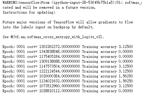
print("Epoch:", '%04d' % (i + 1), "cost=", "{:.9f}".format(loss), "Training accuracy", "{:.5f}".format(acc*100))
print('Optimization Completed')