保本票据
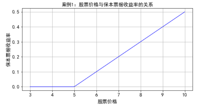
案例1:A金融机构希望推出期限为1年、每份本金为1000元的保本票据。假定目前金融市场存在两个金融资产,一是当前价格为950元、面值为1000元、一年后到期的无风险零息债券;二是基础资产是1股Z股票、执行价格为5元/股、期限为1年的看涨期权,Z股票的当前价格是4.9元/股,股票波动率为20%,该期权的当前市场报价是0.5元。
import numpy as np
import pandas as pd
import matplotlib.pyplot as plt
from pylab import mpl
mpl.rcParams['font.sans-serif']=['SimHei']
mpl.rcParams['axes.unicode_minus']=False
par_ppn=1000.0
price_bond=950.0
par_bond=1000.0
price_z=4.9
K=5.0
T=1.0
price_call=0.5
share_bond=int(par_ppn/price_bond)
share_call=int((par_ppn-share_bond*price_bond)/price_call)
price_z_end=np.linspace(3,10,100)
return_call=np.maximum(price_z_end-K,0)
return_port=share_bond*par_bond+share_call*return_call-par_ppn
plt.figure(figsize=(8,4))
plt.plot(price_z_end,return_port/par_ppn,'b-',lw=1.0)
plt.xlabel(u'股票价格',fontsize=13)
plt.ylabel(u'保本票据收益率',fontsize=13,rotation=90)
plt.xticks(fontsize=13)
plt.yticks(fontsize=13)
plt.title(u'案例1:股票价格与保本票据收益率的关系',fontsize=13)
plt.grid('True')
plt.show()
案例2:假定在2018年12月28日B金融机构推出了期限为半年、金额为1亿元的保本票据,要构造这个保本票据需要两类金融产品,一是高信用评级的债券,金融机构选择了债券到期日最接近保本票据到期日的“16山西债05”地方政府债券;二是在期权合约方面选择了上证50ETF认购期权——50ETF购6月2300合约,该期权到期日是2019年6月26日,期权行权价格为2.3元,期权当天收盘价为0.1649元,期权基础资产上证50ETF基金净值为2.289元,当日上证50指数的收盘点位是2293.10,一张期权对应的合约份数是10000份。
import numpy as np
import pandas as pd
import matplotlib.pyplot as plt
from pylab import mpl
mpl.rcParams['font.sans-serif']=['SimHei']
mpl.rcParams['axes.unicode_minus']=False
principle_ppn=100000000
price_SXbond=101.0809
coupon=0.0259
price_end=100*(1+coupon)
call=0.1649
K=2.3
price_50ETF=2.289
SZ50=2293.10
share_SXbond=10*int(principle_ppn/(10*price_end))
share_SZ50call=int((price_end-price_SXbond)*share_SXbond/(call*10000))
print('需要购买的16山西债05债券数量(单位:张)',share_SXbond)
print('需要购买的上证50ETF认购期权数量(单位:张)',share_SZ50call)
print('达到期权执行价格的上证50指数点位:',round(K*SZ50/price_50ETF,2))
SZ50_increase=np.array([0.1,0.2,0.3,0.4,0.5])
return_ppn=10000*share_SZ50call*(price_50ETF*(1+SZ50_increase)-K)/principle_ppn
print('期权到期日上证50指数上涨10%的保本票据收益率',round(return_ppn[0],6))
print('期权到期日上证50指数上涨20%的保本票据收益率',round(return_ppn[1],6))
print('期权到期日上证50指数上涨30%的保本票据收益率',round(return_ppn[2],6))
print('期权到期日上证50指数上涨40%的保本票据收益率',round(return_ppn[3],6))
print('期权到期日上证50指数上涨50%的保本票据收益率',round(return_ppn[4],6))
SZ50_list=np.linspace(2000,3000,500)
plist_50ETF=SZ50_list*(price_50ETF/SZ50)
rlist_SZ50call=10000*share_SZ50call*np.maximum(plist_50ETF-K,0)
plt.figure(figsize=(8,4))
plt.plot(SZ50_list,rlist_SZ50call/principle_ppn,'b-',lw=1.0)
plt.xlabel(u'上证50指数',fontsize=13)
plt.ylabel(u'保本票据收益率',fontsize=13,rotation=90)
plt.xticks(fontsize=13)
plt.yticks(fontsize=13)
plt.title(u'案例2:上证50指数与保本票据收益率的关系',fontsize=13)
plt.grid('True')
plt.show()

单一期权与单一基础资产的策略
买入备兑看涨期权
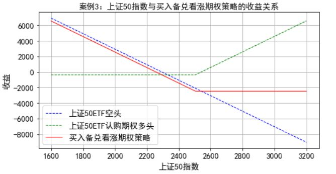
案例3:C金融机构需要构建买入备兑看涨期权策略,策略构建的时间是2018年12月28日,策略中的看涨期权是运用在2019年3月27日到期的、执行价格为2.5元的上证50ETF看涨期权,期权的价格是0.0374元,基础资产是上证50ETF基金,同时,一张期权的基础资产是10000份上证50ETF基金,策略构建当天1份上证50ETF基金的净值是2.289元,上证50指数点位是2293.10。因此,金融机构将运用10000份上证50ETF基金空头头寸和一张上证50ETF看涨期权多头头寸构建买入备兑看涨期权的策略。
import numpy as np
import pandas as pd
import matplotlib.pyplot as plt
from pylab import mpl
mpl.rcParams['font.sans-serif']=['SimHei']
mpl.rcParams['axes.unicode_minus']=False
C=0.0374
K=2.5
P0_ETF=2.289
P0_index=2293.10
Pt_index=np.linspace(1600,3200,500)
Pt_ETF=P0_ETF*Pt_index/P0_index
N_underlying=10000
N_ETF=10000
N_call=1
return_ETF_short=-N_ETF*(Pt_ETF-P0_ETF)
return_call_long=N_call*N_underlying*(np.maximum(Pt_ETF-K,0)-C)
return_covcall_long=return_call_long+return_ETF_short
plt.figure(figsize=(8,4))
plt.plot(Pt_index,return_ETF_short,'b--',label=u'上证50ETF空头',lw=1.0)
plt.plot(Pt_index,return_call_long,'g--',label=u'上证50ETF认购期权多头',lw=1.0)
plt.plot(Pt_index,return_covcall_long,'r-',label=u'买入备兑看涨期权策略',lw=1.0)
plt.xlabel(u'上证50指数',fontsize=13)
plt.ylabel(u'收益',fontsize=13,rotation=90)
plt.xticks(fontsize=13)
plt.yticks(fontsize=13)
plt.title(u'案例3:上证50指数与买入备兑看涨期权策略的收益关系',fontsize=13)
plt.legend(fontsize=13)
plt.legend(fontsize=13)
plt.grid('True')
plt.show()
卖出备兑看涨期权
案例4:D金融机构需要构建卖出备兑看涨期权策略,策略构建的时间是2018年12月28日,策略中的看涨期权是运用在2019年3月27日到期的、执行价格为2.4元的上证50ETF看涨期权,期权的价格是0.0645元,基础资产是上证50ETF基金,同时,一张期权的基础资产是10000份上证50ETF基金,策略构建当天1份上证50ETF基金的净值是2.289元,上证50指数点位是2293.10。金融机构将运用10000份上证50ETF基金多头头寸和一张上证50ETF看涨期权空头头寸构建卖出备兑看涨期权的策略。
import numpy as np
import pandas as pd
import matplotlib.pyplot as plt
from pylab import mpl
mpl.rcParams['font.sans-serif']=['SimHei']
mpl.rcParams['axes.unicode_minus']=False
C=0.0645
K=2.4
P0_ETF=2.289
P0_index=2293.10
Pt_index=np.linspace(1600,3200,500)
Pt_ETF=P0_ETF*Pt_index/P0_index
N_underlying=10000
N_ETF=10000
N_call=1
return_ETF_long=N_ETF*(Pt_ETF-P0_ETF)
return_call_short=N_call*N_underlying*(C-np.maximum(Pt_ETF-K,0))
return_covcall_short=return_call_short+return_ETF_long
plt.figure(figsize=(8,4))
plt.plot(Pt_index,return_ETF_long,'b--',label=u'上证50ETF多头',lw=1.0)
plt.plot(Pt_index,return_call_short,'g--',label=u'上证50ETF认购期权空头',lw=1.0)
plt.plot(Pt_index,return_covcall_short,'r-',label=u'卖出备兑看涨期权策略',lw=1.0)
plt.xlabel(u'上证50指数',fontsize=13)
plt.ylabel(u'收益',fontsize=13,rotation=90)
plt.xticks(fontsize=13)
plt.yticks(fontsize=13)
plt.title(u'案例4:上证50指数与卖出备兑看涨期权策略的收益关系',fontsize=13)
plt.legend(fontsize=13)
plt.legend(fontsize=13)
plt.grid('True')
plt.show()

买入保护看跌期权
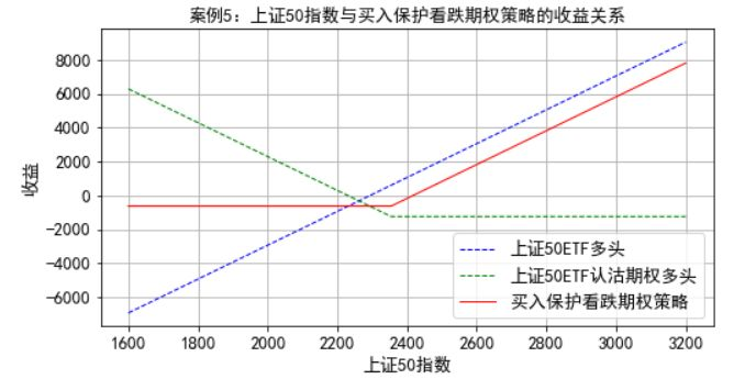
案例5:E金融机构需要构建买入保护看跌期权策略,策略构建的时间是2018年12月28日,策略中的看跌期权是运用在2019年3月27日到期的、执行价格为2.35元的上证50ETF看跌期权,期权的价格是0.1233元,基础资产是上证50ETF基金,同时,一张期权的基础资产是10000份上证50ETF基金,策略构建当天1份上证50ETF基金的净值是2.289元,上证50指数点位是2293.10。金融机构将运用10000份上证50ETF基金多头头寸和一张上证50ETF看跌期权多头头寸构建卖出买入保护看跌期权策略。
import numpy as np
import pandas as pd
import matplotlib.pyplot as plt
from pylab import mpl
mpl.rcParams['font.sans-serif']=['SimHei']
mpl.rcParams['axes.unicode_minus']=False
P=0.1233
K=2.35
P0_ETF=2.289
P0_index=2293.10
Pt_index=np.linspace(1600,3200,500)
Pt_ETF=P0_ETF*Pt_index/P0_index
N_underlying=10000
N_ETF=10000
N_put=1
return_ETF_long=N_ETF*(Pt_ETF-P0_ETF)
return_put_long=N_put*N_underlying*(np.maximum(K-Pt_ETF,0)-P)
return_protput_long=return_put_long+return_ETF_long
plt.figure(figsize=(8,4))
plt.plot(Pt_index,return_ETF_long,'b--',label=u'上证50ETF多头',lw=1.0)
plt.plot(Pt_index,return_put_long,'g--',label=u'上证50ETF认沽期权多头',lw=1.0)
plt.plot(Pt_index,return_protput_long,'r-',label=u'买入保护看跌期权策略',lw=1.0)
plt.xlabel(u'上证50指数',fontsize=13)
plt.ylabel(u'收益',fontsize=13,rotation=90)
plt.xticks(fontsize=13)
plt.yticks(fontsize=13)
plt.title(u'案例5:上证50指数与买入保护看跌期权策略的收益关系',fontsize=13)
plt.legend(fontsize=13)
plt.legend(fontsize=13)
plt.grid('True')
plt.show()
卖出保护看跌期权
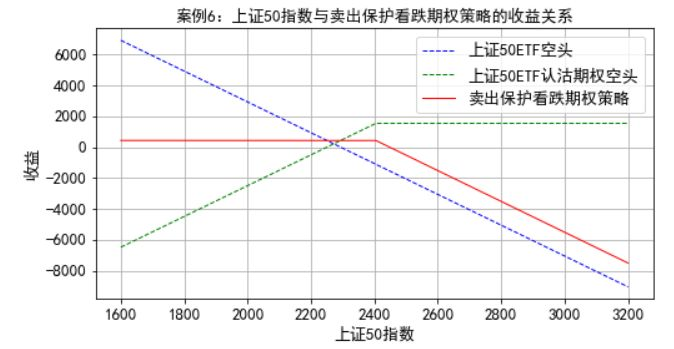
案例6:F金融机构需要构建卖出保护看跌期权策略,策略构建的时间是2018年12月28日,策略中的看跌期权是运用在2019年3月27日到期的、执行价格为2.4元的上证50ETF看跌期权,期权的价格是0.1542元,基础资产是上证50ETF基金,同时,一张期权的基础资产是10000份上证50ETF基金,策略构建当天1份上证50ETF基金的净值是2.289元,上证50指数点位是2293.10。金融机构将运用10000份上证50ETF基金空头头寸和一张上证50ETF看跌期权空头头寸构建卖出保护看跌期权策略。
import numpy as np
import pandas as pd
import matplotlib.pyplot as plt
from pylab import mpl
mpl.rcParams['font.sans-serif']=['SimHei']
mpl.rcParams['axes.unicode_minus']=False
P=0.1542
K=2.4
P0_ETF=2.289
P0_index=2293.10
Pt_index=np.linspace(1600,3200,500)
Pt_ETF=P0_ETF*Pt_index/P0_index
N_underlying=10000
N_ETF=10000
N_put=1
return_ETF_short=-N_ETF*(Pt_ETF-P0_ETF)
return_put_short=N_put*N_underlying*(P-np.maximum(K-Pt_ETF,0))
return_protput_short=return_put_short+return_ETF_short
plt.figure(figsize=(8,4))
plt.plot(Pt_index,return_ETF_short,'b--',label=u'上证50ETF空头',lw=1.0)
plt.plot(Pt_index,return_put_short,'g--',label=u'上证50ETF认沽期权空头',lw=1.0)
plt.plot(Pt_index,return_protput_short,'r-',label=u'卖出保护看跌期权策略',lw=1.0)
plt.xlabel(u'上证50指数',fontsize=13)
plt.ylabel(u'收益',fontsize=13,rotation=90)
plt.xticks(fontsize=13)
plt.yticks(fontsize=13)
plt.title(u'案例6:上证50指数与卖出保护看跌期权策略的收益关系',fontsize=13)
plt.legend(fontsize=13)
plt.legend(fontsize=13)
plt.grid('True')
plt.show()
价差交易策略
牛市价差策略
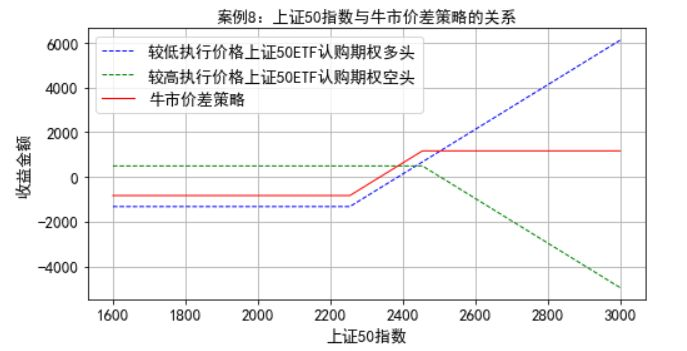
案例8:H金融机构需要构建牛市价差策略,策略构建的时间是2018年12月28日,两个看涨期权均是在2019年3月27日到期的上证50ETF期权,其中一个是较低的执行价格2.25元,期权价格是0.1325元,另一个期权是较高的执行价格2.45元,期权价格是0.0494元,策略构建当天上证50ETF基金的净值是2.289元,上证50指数点位是2293.10。金融机构运用一张执行价格2.25元的上证50ETF看涨期权多头头寸和一张执行价格2.45元的上证50ETF看涨期权空头头寸构建牛市价差策略。
import numpy as np
import pandas as pd
import matplotlib.pyplot as plt
from pylab import mpl
mpl.rcParams['font.sans-serif']=['SimHei']
mpl.rcParams['axes.unicode_minus']=False
K1=2.25
K2=2.45
C1=0.1325
C2=0.0494
P0_ETF=2.289
P0_index=2293.10
Pt_index=np.linspace(1600,3000,500)
Pt_ETF=P0_ETF*Pt_index/P0_index
N1=1
N2=1
N_underlying=10000
return_call1_long=N1*N_underlying*(np.maximum(Pt_ETF-K1,0)-C1)
return_call2_short=N2*N_underlying*(C2-np.maximum(Pt_ETF-K2,0))
return_bullspread=return_call1_long+return_call2_short
plt.figure(figsize=(8,4))
plt.plot(Pt_index,return_call1_long,'b--',label=u'较低执行价格上证50ETF认购期权多头',lw=1.0)
plt.plot(Pt_index,return_call2_short,'g--',label=u'较高执行价格上证50ETF认购期权空头',lw=1.0)
plt.plot(Pt_index,return_bullspread,'r-',label=u'牛市价差策略',lw=1.0)
plt.xlabel(u'上证50指数',fontsize=13)
plt.ylabel(u'收益金额',fontsize=13,rotation=90)
plt.xticks(fontsize=13)
plt.yticks(fontsize=13)
plt.title(u'案例8:上证50指数与牛市价差策略的关系',fontsize=13)
plt.legend(fontsize=13)
plt.legend(fontsize=13)
plt.grid('True')
plt.show()
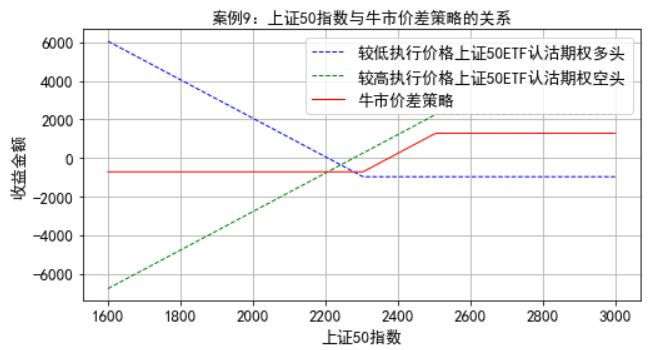
案例9:I金融机构希望运用看跌期权构建牛市价差策略,策略构建的时间是2018年12月28日,两个看跌期权均是在2019年3月27日到期的上证50ETF期权,其中一个是较低的执行价格2.3元,期权价格是0.0972元,另一个期权是较高的执行价格2.5元,期权价格是0.2255元,策略构建当天上证50ETF基金的净值是2.289元,上证50指数点位是2293.10。金融机构运用一张执行价格2.3元的上证50ETF看跌期权多头头寸和一张执行价格2.5元的上证50ETF看跌期权空头头寸构建牛市价差策略。
import numpy as np
import pandas as pd
import matplotlib.pyplot as plt
from pylab import mpl
mpl.rcParams['font.sans-serif']=['SimHei']
mpl.rcParams['axes.unicode_minus']=False
K1=2.3
K2=2.5
P1=0.0972
P2=0.2255
P0_ETF=2.289
P0_index=2293.10
Pt_index=np.linspace(1600,3000,500)
Pt_ETF=P0_ETF*Pt_index/P0_index
N1=1
N2=1
N_underlying=10000
return_put1_long=N1*N_underlying*(np.maximum(K1-Pt_ETF,0)-P1)
return_put2_short=N2*N_underlying*(P2-np.maximum(K2-Pt_ETF,0))
return_bullspread=return_put1_long+return_put2_short
plt.figure(figsize=(8,4))
plt.plot(Pt_index,return_put1_long,'b--',label=u'较低执行价格上证50ETF认沽期权多头',lw=1.0)
plt.plot(Pt_index,return_put2_short,'g--',label=u'较高执行价格上证50ETF认沽期权空头',lw=1.0)
plt.plot(Pt_index,return_bullspread,'r-',label=u'牛市价差策略',lw=1.0)
plt.xlabel(u'上证50指数',fontsize=13)
plt.ylabel(u'收益金额',fontsize=13,rotation=90)
plt.xticks(fontsize=13)
plt.yticks(fontsize=13)
plt.title(u'案例9:上证50指数与牛市价差策略的关系',fontsize=13)
plt.legend(fontsize=13)
plt.legend(fontsize=13)
plt.grid('True')
plt.show()
熊市价差策略
案例10:J金融机构需要构建牛市价差策略,策略构建的时间是2018年12月28日,两个看跌期权均是在2019年3月27日到期的上证50ETF期权,其中一个是较低的执行价格2.25元,期权价格是0.0734元,另一个期权是较高的执行价格2.55元,期权价格是0.2683元,策略构建当天上证50ETF基金的净值是2.289元,上证50指数点位是2293.10。金融机构运用一张执行价格2.25元的上证50ETF看跌期权空头头寸和一张执行价格2.55元的上证50ETF看跌期权多头头寸构建熊市价差策略。
import numpy as np
import pandas as pd
import matplotlib.pyplot as plt
from pylab import mpl
mpl.rcParams['font.sans-serif']=['SimHei']
mpl.rcParams['axes.unicode_minus']=False
K1=2.25
K2=2.55
P1=0.0734
P2=0.2683
P0_ETF=2.289
P0_index=2293.10
Pt_index=np.linspace(1600,3000,500)
Pt_ETF=P0_ETF*Pt_index/P0_index
N1=1
N2=1
N_underlying=10000
return_put1_short=N1*N_underlying*(P1-np.maximum(K1-Pt_ETF,0))
return_put2_long=N2*N_underlying*(np.maximum(K2-Pt_ETF,0)-P2)
return_bearspread=return_put1_short+return_put2_long
plt.figure(figsize=(8,4))
plt.plot(Pt_index,return_put1_short,'b--',label=u'较低执行价格上证50ETF认沽期权空头',lw=1.0)
plt.plot(Pt_index,return_put2_long,'g--',label=u'较高执行价格上证50ETF认沽期权多头',lw=1.0)
plt.plot(Pt_index,return_bearspread,'r-',label=u'熊市价差策略',lw=1.0)
plt.xlabel(u'上证50指数',fontsize=13)
plt.ylabel(u'收益金额',fontsize=13,rotation=90)
plt.xticks(fontsize=13)
plt.yticks(fontsize=13)
plt.title(u'案例10:上证50指数与熊市价差策略的关系',fontsize=13)
plt.legend(fontsize=13)
plt.legend(fontsize=13)
plt.grid('True')
plt.show()

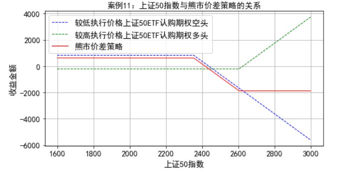
案例11:K金融机构希望运用看涨期权构建熊市价差策略,策略构建的时间是2018年12月28日,两个看涨期权均是在2019年3月27日到期的上证50ETF期权,其中一个是较低的执行价格2.35元,期权价格是0.083元,另一个期权是较高的执行价格2.6元,期权价格是0.0203元,策略构建当天上证50ETF基金的净值是2.289元,上证50指数点位是2293.10。金融机构运用一张执行价格2.35元的上证50ETF看涨期权空头头寸和一张执行价格2.6元的上证50ETF看涨期权多头头寸构建熊市价差策略。
import numpy as np
import pandas as pd
import matplotlib.pyplot as plt
from pylab import mpl
mpl.rcParams['font.sans-serif']=['SimHei']
mpl.rcParams['axes.unicode_minus']=False
K1=2.35
K2=2.6
P1=0.083
P2=0.0203
P0_ETF=2.289
P0_index=2293.10
Pt_index=np.linspace(1600,3000,500)
Pt_ETF=P0_ETF*Pt_index/P0_index
N1=1
N2=1
N_underlying=10000
return_call1_short=N1*N_underlying*(P1-np.maximum(Pt_ETF-K1,0))
return_call2_long=N2*N_underlying*(np.maximum(Pt_ETF-K2,0)-P2)
return_bearspread=return_call1_short+return_call2_long
plt.figure(figsize=(8,4))
plt.plot(Pt_index,return_call1_short,'b--',label=u'较低执行价格上证50ETF认购期权空头',lw=1.0)
plt.plot(Pt_index,return_call2_long,'g--',label=u'较高执行价格上证50ETF认购期权多头',lw=1.0)
plt.plot(Pt_index,return_bearspread,'r-',label=u'熊市价差策略',lw=1.0)
plt.xlabel(u'上证50指数',fontsize=13)
plt.ylabel(u'收益金额',fontsize=13,rotation=90)
plt.xticks(fontsize=13)
plt.yticks(fontsize=13)
plt.title(u'案例11:上证50指数与熊市价差策略的关系',fontsize=13)
plt.legend(fontsize=13)
plt.legend(fontsize=13)
plt.grid('True')
plt.show()
盒式价差策略
案例12:L金融机构希望构建盒式价差策略,构建策略的时间是2018年12月28日,运用的4个期权均是在2019年3月27日到期的上证50ETF期权,具体的期权信息及策略如下表所示
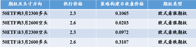
策略构建当天,上证50ETF基金的净值是2.289元,上证50指数点位是2293.10。
import numpy as np
import pandas as pd
import matplotlib.pyplot as plt
from pylab import mpl
mpl.rcParams['font.sans-serif']=['SimHei']
mpl.rcParams['axes.unicode_minus']=False
K1=2.3
K2=2.6
C1=0.1065
C2=0.0203
P1=0.0972
P2=0.3107
P0_ETF=2.289
P0_index=2293.10
Pt_index=np.linspace(1600,3000,500)
Pt_ETF=P0_ETF*Pt_index/P0_index
N_call=1
N_put=1
N_underlying=10000
return_call1_long=N_call*N_underlying*(np.maximum(Pt_ETF-K1,0)-C1)
return_call2_short=N_call*N_underlying*(C2-np.maximum(Pt_ETF-K2,0))
return_put2_long=N_put*N_underlying*(np.maximum(K2-Pt_ETF,0)-P2)
return_put1_short=N_put*N_underlying*(P1-np.maximum(K1-Pt_ETF,0))
return_boxspread=return_call1_long+return_call2_short+return_put2_long+return_put1_short
plt.figure(figsize=(8,5))
plt.plot(Pt_index,return_call1_long,'b--',label=u'较低执行价格上证50ETF认购期权多头',lw=1.0)
plt.plot(Pt_index,return_call2_short,'g--',label=u'较高执行价格上证50ETF认购期权空头',lw=1.0)
plt.plot(Pt_index,return_put1_short,'c--',label=u'较低执行价格上证50ETF认沽期权多头',lw=1.0)
plt.plot(Pt_index,return_put2_long,'m--',label=u'较高执行价格上证50ETF认沽期权空头',lw=1.0)
plt.plot(Pt_index,return_boxspread,'r-',label=u'盒式价差策略',lw=1.0)
plt.xlabel(u'上证50指数',fontsize=13)
plt.ylabel(u'收益金额',fontsize=13,rotation=90)
plt.xticks(fontsize=13)
plt.yticks(fontsize=13)
plt.title(u'案例12:上证50指数与盒式价差策略的关系',fontsize=13)
plt.legend(fontsize=13)
plt.legend(fontsize=13)
plt.grid('True')
plt.show()

组合策略
跨式组合策略
案例15:P金融机构希望构建底部跨式组合策略,构建策略的时间是2018年12月18日,策略中运用的两个期权均是在2019年6月26日到期的、执行价格为2.4元的上证50ETF期权,其中,一只看涨期权的价格是0.1745元,另一只看跌期权的价格是0.1106元,当天的上证50ETF净值是2.394元,上证50指数的收盘点位2397.87。金融机构运用一张执行价格2.4元的上证50ETF看涨期权多头头寸、一张执行价格也是2.4元的上证50ETF看跌期权多头头寸构建底部跨式组合策略。
import numpy as np
import pandas as pd
import matplotlib.pyplot as plt
from pylab import mpl
mpl.rcParams['font.sans-serif']=['SimHei']
mpl.rcParams['axes.unicode_minus']=False
K=2.4
C=0.1745
P=0.1106
P0_ETF=2.394
P0_index=2397.87
Pt_index=np.linspace(1800,3000,500)
Pt_ETF=P0_ETF*Pt_index/P0_index
N_call=1
N_put=1
N_underlying=10000
return_call_long=N_call*N_underlying*(np.maximum(Pt_ETF-K,0)-C)
return_put_long=N_put*N_underlying*(np.maximum(K-Pt_ETF,0)-P)
return_straddle=return_call_long+return_put_long
plt.figure(figsize=(8,4))
plt.plot(Pt_index,return_call_long,'b--',label=u'上证50ETF认购期权多头',lw=1)
plt.plot(Pt_index,return_put_long,'g--',label=u'上证50ETF认沽期权多头',lw=1)
plt.plot(Pt_index,return_straddle,'r-',label=u'底部跨式组合策略',lw=1)
plt.xlabel(u'上证50指数',fontsize=13)
plt.ylabel(u'收益金额',fontsize=13,rotation=90)
plt.xticks(fontsize=13)
plt.yticks(fontsize=13)
plt.title(u'案例15:上证50指数与底部跨式组合策略的关系',fontsize=13)
plt.legend(fontsize=13)
plt.grid('True')
plt.show()

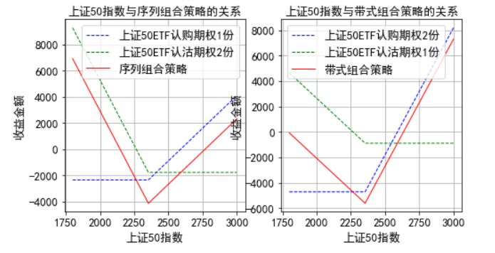
序列组合策略与带式组合策略
案例17:Q金融机构希望构建序列组合和带式组合策略,构建策略的时间是2018年12月18日,策略中运用的两个期权均是在2019年6月26日到期的、执行价格为2.35元的上证50ETF期权,其中,一只看涨期权的价格是0.2360元,另一只看跌期权的价格是0.0893元,当天的上证50ETF净值是2.394元,上证50指数的收盘点位2397.87。金融机构运用一张执行价格2.35元的上证50ETF看涨期权多头头寸、两张执行价格也是2.35元的上证50ETF看跌期权多头头寸构建序列组合策略;同时,又运用两张上证50ETF看涨期权多头头寸、一张上证50ETF看跌期权多头头寸构建带式组合策略。
import numpy as np
import pandas as pd
import matplotlib.pyplot as plt
from pylab import mpl
mpl.rcParams['font.sans-serif']=['SimHei']
mpl.rcParams['axes.unicode_minus']=False
K=2.35
C=0.2360
P=0.0893
P0_ETF=2.394
P0_index=2397.87
Pt_index=np.linspace(1800,3000,500)
Pt_ETF=P0_ETF*Pt_index/P0_index
N_callstrip=1
N_callstrap=2
N_putstrip=2
N_putstrap=1
N_underlying=10000
return_callstrip=N_callstrip*N_underlying*(np.maximum(Pt_ETF-K,0)-C)
return_putstrip=N_putstrip*N_underlying*(np.maximum(K-Pt_ETF,0)-P)
return_strip=return_callstrip+return_putstrip
return_callstrap=N_callstrap*N_underlying*(np.maximum(Pt_ETF-K,0)-C)
return_putstrap=N_putstrap*N_underlying*(np.maximum(K-Pt_ETF,0)-P)
return_strap=return_callstrap+return_putstrap
plt.figure(figsize=(8,4))
plt.subplot(1,2,1)
plt.plot(Pt_index,return_callstrip,'b--',label=u'上证50ETF认购期权1份',lw=1)
plt.plot(Pt_index,return_putstrip,'g--',label=u'上证50ETF认沽期权2份',lw=1)
plt.plot(Pt_index,return_strip,'r-',label=u'序列组合策略',lw=1)
plt.xlabel(u'上证50指数',fontsize=13)
plt.ylabel(u'收益金额',fontsize=13,rotation=90)
plt.xticks(fontsize=13)
plt.yticks(fontsize=13)
plt.title(u'上证50指数与序列组合策略的关系',fontsize=13)
plt.legend(loc=0,fontsize=13)
plt.grid('True')
plt.subplot(1,2,2)
plt.plot(Pt_index,return_callstrap,'b--',label=u'上证50ETF认购期权2份',lw=1)
plt.plot(Pt_index,return_putstrap,'g--',label=u'上证50ETF认沽期权1份',lw=1)
plt.plot(Pt_index,return_strap,'r-',label=u'带式组合策略',lw=1)
plt.xlabel(u'上证50指数',fontsize=13)
plt.ylabel(u'收益金额',fontsize=13,rotation=90)
plt.xticks(fontsize=13)
plt.yticks(fontsize=13)
plt.title(u'上证50指数与带式组合策略的关系',fontsize=13)
plt.legend(loc=0,fontsize=13)
plt.grid('True')
宽跨式组合策略
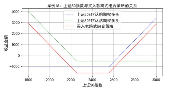
案例18:R金融机构希望构建买入宽跨式组合策略,构建策略的时间是2018年12月18日,策略中运用的两个期权均是在2019年6月26日到期的、执行价格为2.25元的看跌期权,价格是0.0545元,另一只是执行价格为2.55元的看涨期权,期权价格是0.1077元。当天的上证50ETF净值是2.394元,上证50指数的收盘点位2397.87。金融机构运用一张执行价格2.25元的上证50ETF看跌期权多头头寸、一张执行价格是2.55元的上证50ETF看涨期权多头头寸构建买入宽跨式组合策略。
import numpy as np
import pandas as pd
import matplotlib.pyplot as plt
from pylab import mpl
mpl.rcParams['font.sans-serif']=['SimHei']
mpl.rcParams['axes.unicode_minus']=False
K1=2.25
K2=2.55
C=0.1077
P=0.0545
P0_ETF=2.394
P0_index=2397.87
Pt_index=np.linspace(1800,3000,500)
Pt_ETF=P0_ETF*Pt_index/P0_index
N_call=1
N_put=1
N_underlying=10000
return_call=N_call*N_underlying*(np.maximum(Pt_ETF-K2,0)-C)
return_put=N_put*N_underlying*(np.maximum(K1-Pt_ETF,0)-P)
return_strangle=return_call+return_put
plt.figure(figsize=(8,4))
plt.plot(Pt_index,return_call,'b--',label=u'上证50ETF认购期权多头',lw=1)
plt.plot(Pt_index,return_put,'g--',label=u'上证50ETF认沽期权多头',lw=1)
plt.plot(Pt_index,return_strangle,'r-',label=u'买入宽跨式组合策略',lw=1)
plt.xlabel(u'上证50指数',fontsize=13)
plt.ylabel(u'收益金额',fontsize=13,rotation=90)
plt.xticks(fontsize=13)
plt.yticks(fontsize=13)
plt.title(u'案例18:上证50指数与买入款跨式组合策略的关系',fontsize=13)
plt.legend(fontsize=13)
plt.grid('True')
plt.show()