第一次编程作业

function A = warmUpExercise()
%WARMUPEXERCISE Example function in octave
%   A = WARMUPEXERCISE() is an example function that returns the 5x5 identity matrix

A = [];
% ============= YOUR CODE HERE ==============
% Instructions: Return the 5x5 identity matrix 
%               In octave, we return values by defining which variables
%               represent the return values (at the top of the file)
%               and then set them accordingly. 



A = eye(5);



% ===========================================


end


function J = computeCost(X, y, theta)
%COMPUTECOST Compute cost for linear regression
%   J = COMPUTECOST(X, y, theta) computes the cost of using theta as the
%   parameter for linear regression to fit the data points in X and y

% Initialize some useful values
m = length(y); % number of training examples

% You need to return the following variables correctly 
J = 0;

% ====================== YOUR CODE HERE ======================
% Instructions: Compute the cost of a particular choice of theta
%               You should set J to the cost.

predictions = X*theta;
sqrErrors = (predictions - y) .^2;%每个元素取平方
J = 1/(2*m) *sum(sqrErrors);



% =========================================================================

end

function plotData(x, y)
%PLOTDATA Plots the data points x and y into a new figure 
%   PLOTDATA(x,y) plots the data points and gives the figure axes labels of
%   population and profit.

figure; % open a new figure window

% ====================== YOUR CODE HERE ======================
% Instructions: Plot the training data into a figure using the 
%               "figure" and "plot" commands. Set the axes labels using
%               the "xlabel" and "ylabel" commands. Assume the 
%               population and revenue data have been passed in
%               as the x and y arguments of this function.
%
% Hint: You can use the 'rx' option with plot to have the markers
%       appear as red crosses. Furthermore, you can make the
%       markers larger by using plot(..., 'rx', 'MarkerSize', 10);

plot(x,y,'rx','MarkerSize',10);% rx 红色的 叉号 ‘x’。大小为10
ylabel('Profit in $10,000s');
xlabel('population of City in 10,000s');



% ============================================================

end

执行ex1 回依次执行所有不得.m文件，直至结束。若想中途停止shift+ctrl+c

function [theta, J_history] = gradientDescent(X, y, theta, alpha, num_iters)
%GRADIENTDESCENT Performs gradient descent to learn theta
%   theta = GRADIENTDESCENT(X, y, theta, alpha, num_iters) updates theta by 
%   taking num_iters gradient steps with learning rate alpha

% Initialize some useful values
m = length(y); % number of training examples
J_history = zeros(num_iters, 1);

for iter = 1:num_iters

    % ====================== YOUR CODE HERE ======================
    % Instructions: Perform a single gradient step on the parameter vector
    %               theta. 
    %
    % Hint: While debugging, it can be useful to print out the values
    %       of the cost function (computeCost) and gradient here.
    %

    theta1=theta(1,1)-alpha/m*sum(X*theta-y);
    theta2=theta(2,1)-alpha/m*sum((X*theta-y) .* X(:,2));
    theta(1,1)=theta1;
    theta(2,1)=theta2;


    % ============================================================

    % Save the cost J in every iteration    
    J_history(iter) = computeCost(X, y, theta);

end

end

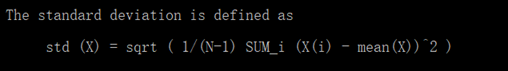
function [X_norm, mu, sigma] = featureNormalize(X)
%FEATURENORMALIZE Normalizes the features in X 
%   FEATURENORMALIZE(X) returns a normalized version of X where
%   the mean value of each feature is 0 and the standard deviation
%   is 1. This is often a good preprocessing step to do when
%   working with learning algorithms.

% You need to set these values correctly
X_norm = X;
mu = zeros(1, size(X, 2));
sigma = zeros(1, size(X, 2));

% ====================== YOUR CODE HERE ======================
% Instructions: First, for each feature dimension, compute the mean
%               of the feature and subtract it from the dataset,
%               storing the mean value in mu. Next, compute the 
%               standard deviation of each feature and divide
%               each feature by it's standard deviation, storing
%               the standard deviation in sigma. 
%
%               Note that X is a matrix where each column is a 
%               feature and each row is an example. You need 
%               to perform the normalization separately for 
%               each feature. 
%
% Hint: You might find the 'mean' and 'std' functions useful.
%       

m = size(X,2)%列数
for i=1:m,
   mu(i)=mean(X(:,i))%X第i列的平均数
   sigma(i) =std(X(:,i))%X第i列的标准差
end

X_norm =(X_norm-mu)./sigma;%这里同样是对应元素的运算

% ============================================================

end

元素间的加减，点乘、除要保证列数一致
>> A =[1 2;3 4;5 6]
A =

   1   2
   3   4
   5   6

>> B = [1 2]
B =

1 2

>> A-B
ans =

   0   0
   2   2
   4   4

>> A./B
ans =

   1   1
   3   2
   5   3

function [theta, J_history] = gradientDescentMulti(X, y, theta, alpha, num_iters)
%GRADIENTDESCENTMULTI Performs gradient descent to learn theta
%   theta = GRADIENTDESCENTMULTI(x, y, theta, alpha, num_iters) updates theta by
%   taking num_iters gradient steps with learning rate alpha

% Initialize some useful values
m = length(y); % number of training examples
J_history = zeros(num_iters, 1);
temp = theta;
for iter = 1:num_iters

    % ====================== YOUR CODE HERE ======================
    % Instructions: Perform a single gradient step on the parameter vector
    %               theta. 
    %
    % Hint: While debugging, it can be useful to print out the values
    %       of the cost function (computeCostMulti) and gradient here.
    %
    for i =1:length(theta),
        temp(i,1) = temp(i,1)-alpha/m*sum((X*theta-y).*X(:,i));
    end
    theta = temp;    

    % ============================================================

    % Save the cost J in every iteration    
    J_history(iter) = computeCostMulti(X, y, theta);

end

end

length(v) 这个命令将返回最大维度的大小

function [theta] = normalEqn(X, y)
%NORMALEQN Computes the closed-form solution to linear regression 
%   NORMALEQN(X,y) computes the closed-form solution to linear 
%   regression using the normal equations.

theta = zeros(size(X, 2), 1);

% ====================== YOUR CODE HERE ======================
% Instructions: Complete the code to compute the closed form solution
%               to linear regression and put the result in theta.
%

% ---------------------- Sample Solution ----------------------

theta = pinv(X'*X)*X'*y;


% -------------------------------------------------------------


% ============================================================

end

function J = computeCostMulti(X, y, theta)
%COMPUTECOSTMULTI Compute cost for linear regression with multiple variables
%   J = COMPUTECOSTMULTI(X, y, theta) computes the cost of using theta as the
%   parameter for linear regression to fit the data points in X and y

% Initialize some useful values
m = length(y); % number of training examples

% You need to return the following variables correctly 
J = 0;

% ====================== YOUR CODE HERE ======================
% Instructions: Compute the cost of a particular choice of theta
%               You should set J to the cost.

predictions = X*theta;
sqrErrors = (predictions -y).^2;
J = 1/(2*m)*sum(sqrErrors);



% =========================================================================

end