时间序列分析(二）

imetime series data mining主要包括decompose（分析数据的各个成分，例如趋势，周期性），prediction（预测未来的值），classification（对有序数据序列的feature提取与分类），clustering（相似数列聚类）等。时序数据prediction（forecast，预测）使用最广泛的两个算法： Holt-Winters 和 ARIMA。其它的常用函数说明如下：

stats::ts() --生成时序对象
stats::start() --返回时间序列的开始时间
stats::end() --返回时间序列的开始时间
stats::frequency --返回时间序列中时间点的个数
stats::window() --对时间序列取子集

graphics::plot() --画出时间序列拆线图
stats::monthplot() --画出时序中的季节项
forecast::seasonplot --生成季节图

stats::stl() -- 用 LOESS光滑将时序分解为季节项、趋势项和随机项。局限之处——只能处理相加模型
stats::decompose() -- 对相加与相乘模型都可以直接进行季节分解

forecast::ma() -- 拟合一个简单的移动平均模型
stats::HoltWinters() -- 三次平滑指数法，拟合指数平常模型
forecast::ets() -- 拟合指数平滑模型，同时也可以自动选取最优模型
forecast::accuracy() -- 返回时序的拟合优度度量

tseries::adf.test() -- 对序列做ADF检验以判断其是否平稳
stats::lag() -- 返回取过指定滞后项后的时序
base::diff() -- 返回取过滞后项和差分后的序列
forecast::ndiffs() -- 找到最优差分次数以移除序列中的趋势项
forecast::acf() -- 估计自相关函数
forecast::pacf() -- 估计偏自相关函数

stats::arima() -- 似合 ARIMA模型
forecast::auto.arima() --自动选择 ARIMA模型，可能不准确
forecast::forecast() --预测时序的未来值

stats::Box.test() -- 进行Ljung-Box 检验以判断模型的残差是否独立
tseries::bds.test() -- 进行BDS检验以判断序列中的随机变量是否服从独立分布

stats::ts()：生成时序对象

ts(data, frequency=n, start=x, end=y, names=c(a,b,c,...))

data: 观察到的时间序列值的向量或矩阵。
frequency: 频次，n=1 为年， n=4为季度，n=7 为周， n=12 为月等
start: 起始时点

> t <- ts(testSrc$tp,start = c(2016,1),frequency= 12)
> start(t)
[1] 2016    1
> end(t)
[1] 2017   12
> frequency(t)
[1] 12

按天时间段

> library(zoo)
> zoo <- zoo(testSrc$dp,order.by = as.Date(as.character(testSrc$biztime), format='%Y-%m-%d'))
> ts <- ts(zoo)
> str(ts)
 Time-Series [1:742] from 1 to 742: 62772 57541 59310 66895 71020 ...
 - attr(*, "index")= Date[1:742], format: "2016-01-01" "2016-01-02" "2016-01-03" "2016-01-04" ...

另一种写法：

xl<- ts(testSrc$dp,start=c(2016,01,01),frequency=365)
str(xl)

stats::decompose() 对相加与相乘模型都可以直接进行季节分解

decompose(x, type = c("additive", "multiplicative"), filter = NULL)

xl<- ts(testSrc$dp,start=c(2016,01,01),frequency=365)

##季节分解
ml <- decompose(xl,c("multiplicative"))
plot(ml)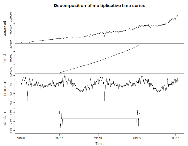

在分解季节成分的基础上，如果有需要的话，我们可以对时间序列进行季节因素调整，将这一部分信息从原始数据中去除。

xl<- ts(testSrc$dp,start=c(2016,01,01),frequency=365)

##季节分解
ml <- decompose(xl,c("multiplicative"))
plot(ml)

data2 <- xl - ml$seasonal
par(mfrow=c(1,2))
plot(xl)
plot(data2)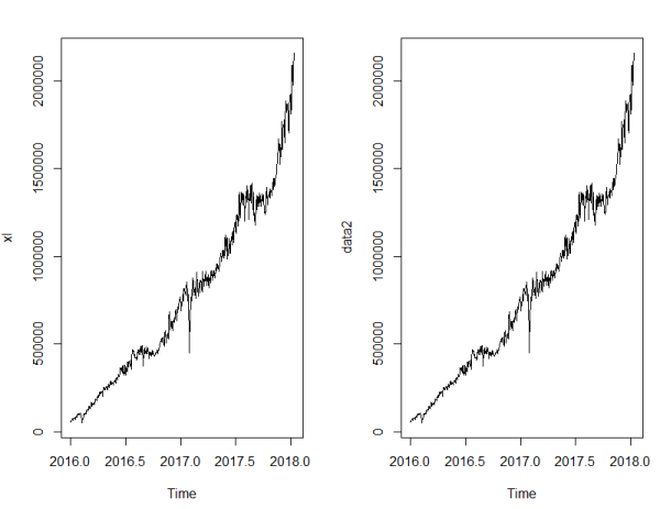

forecast::ets()：拟合指数平滑模型

ets(ts, model="ZZZ",.....)

限制模型的字母有三个。第一个字母代表误差项，第二个字母代表趋势项，第三个字母则代表季节项。
可选的字母包括：相加模型（A)、相乘模型（M)、无（N）、自动选择（Z）。

通过ets()函数自动选取对原始数据拟合优度最高的模型。

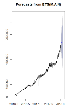
> library(forecast)
> x <- ets(data2)
Warning message:
In ets(data2) :
  I can't handle data with frequency greater than 24. Seasonality will be ignored. Try stlf() if you need seasonal forecasts.
> x
ETS(M,A,N) 

Call:
 ets(y = data2) 

  Smoothing parameters:
    alpha = 0.9999 
    beta  = 1e-04 

  Initial states:
    l = 60125.3605 
    b = 1757.7865 

  sigma:  0.0459

     AIC     AICc      BIC 
20049.03 20049.12 20072.08 
> plot(x)

效果图
预测

> pre <- forecast(x,h=30)
> pre$mean
Time Series:
Start = c(2018, 13) 
End = c(2018, 42) 
Frequency = 365 
 [1] 2159078 2160914 2162751 2164588 2166424 2168261 2170097 2171934 2173771 2175607 2177444 2179281 2181117 2182954 2184790
[16] 2186627 2188464 2190300 2192137 2193974 2195810 2197647 2199483 2201320 2203157 2204993 2206830 2208667 2210503 2212340
> plot(pre)