原文链接:http://tecdat.cn/?p=19688
在引入copula时,大家普遍认为copula很有趣,因为它们允许分别对边缘分布和相依结构进行建模。
copula建模边缘和相依关系
给定一些边缘分布函数和一个copula,那么我们可以生成一个多元分布函数,其中的边缘是前面指定的。
考虑一个二元对数正态分布
-
-
> library(mnormt)
-
> set.seed(1)
-
> Z=exp(rmnorm(25,MU,SIGMA))
我们可以从边缘分布开始。
-
-
meanlog sdlog
-
1.168 0.930
-
(0.186 ) (0.131 )
-
-
meanlog sdlog
-
2.218 1.168
-
(0.233 ) (0.165 )
基于这些边缘分布,并考虑从该伪随机样本获得的copula参数的最大似然估计值,从数值上讲,我们得到
-
-
> library(copula)
-
-
> Copula() estimation based on 'maximum likelihood'
-
and a sample of size 25.
-
Estimate Std. Error z value Pr(>|z|)
-
rho.1 0.86530 0.03799 22.77
但是,由于相依关系是边缘分布的函数,因此我们没有对相依关系进行单独处理。如果考虑全局优化问题,则结果会有所不同。可以得出密度
-
-
> optim(par=c(0,0,1,1,0),fn=LogLik)$par
-
[1] 1.165 2.215 0.923 1.161 0.864
差别不大,但估计量并不相同。从统计的角度来看,我们几乎无法分别处理边缘和相依结构。我们应该记住的另一点是,边际分布可能会错误指定。例如,如果我们假设指数分布,
-
-
fitdistr(Z[,1],"exponential")
-
rate
-
0.222
-
(0.044 )
-
fitdistr(Z[,2],"exponential"
-
rate
-
0.065
-
(0.013 )
高斯copula的参数估计
-
-
Copula() estimation based on 'maximum likelihood'
-
and a sample of size 25.
-
Estimate Std. Error z value Pr(>|z|)
-
rho.1 0.87421 0.03617 24.17 <2e-16 ***
-
-
Signif. codes: 0 '***' 0.001 '**' 0.01 '*' 0.05 '.' 0.1 ' ' 1
-
The maximized loglikelihood is 15.4
-
Optimization converged
由于我们错误地指定了边缘分布,因此我们无法获得统一的边缘。如果我们使用上述代码生成大小为500的样本,
-
-
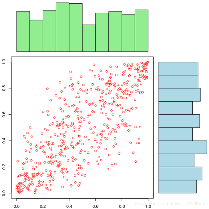
barplot(counts, axes=FALSE,col="light blue"
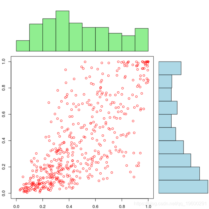
如果边缘分布被很好地设定时,我们可以清楚地看到相依结构依赖于边缘分布,
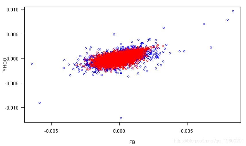
copula模拟股市中相关随机游走
接下来我们用copula函数模拟股市中的相关随机游走
-
#*****************************************************************
-
# 载入历史数据
-
#******************************************************************
-
-
load.packages('quantmod')
-
-
data$YHOO = getSymbol.intraday.google('YHOO', 'NASDAQ', 60, '15d')
-
data$FB = getSymbol.intraday.google('FB', 'NASDAQ', 60, '15d')
-
bt.prep(data, align='remove.na')
-
-
-
#*****************************************************************
-
# 生成模拟
-
#******************************************************************
-
-
rets = diff(log(prices))
-
-
# 绘制价格
-
matplot(exp(apply(rets,2,cumsum)), type='l')

-
# 可视化分布的辅助函数
-
-
# 检查Copula拟合的Helper函数
-
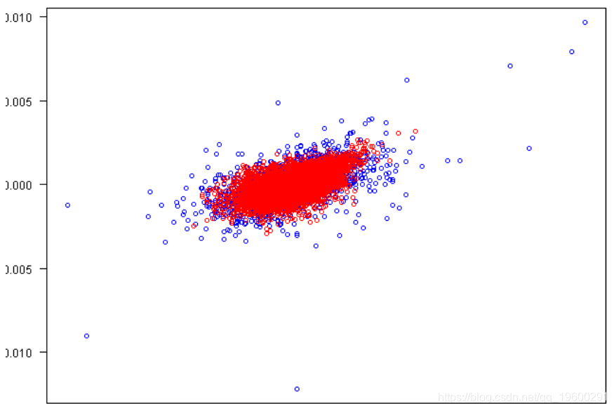
# 模拟图与实际图
-
-
plot(rets[,1], rets[,2], xlab=labs[1], ylab=labs[2], col='blue', las=1)
-
points(fit.sim[,1], fit.sim[,2], col='red')
-
-
# 比较模拟和实际的统计数据
-
temp = matrix(0,nr=5,nc=2)
-
-
print(round(100*temp,2))
-
-
# 检查收益率是否来自相同的分布
-
for (i in 1:2) {
-
print(labs[i])
-
print(ks.test(rets[,i], fit.sim[i]))
-
-
-
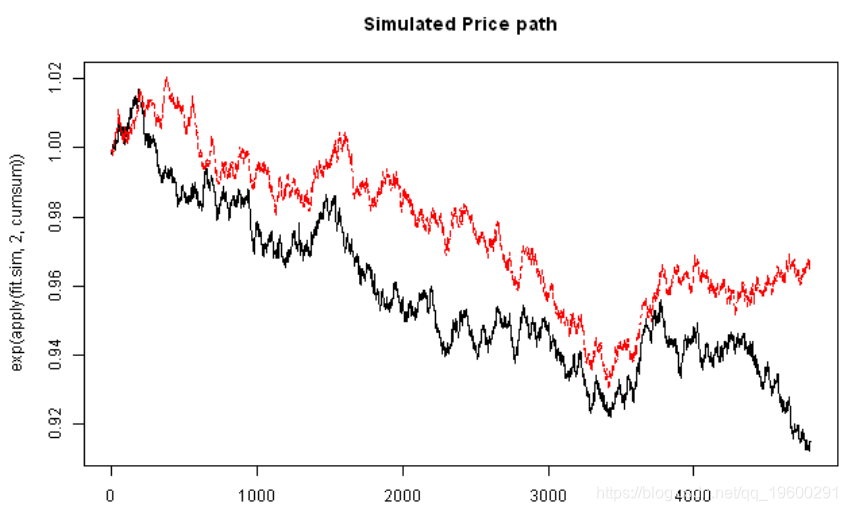
# 绘制模拟价格路径
-
matplot(exp(apply(fit.sim,2,cumsum)), type='l', main='Simulated Price path')
-
-
-
# 拟合Copula
-
load.packages('copula')
-
-
# 通过组合拟合边缘和拟合copula创建自定义分布
-
margins=c("norm","norm")
-
apply(rets,2,function(x) list(mean=mean(x), sd=sd(x)))
-
-
-
# 从拟合分布模拟
-
rMvdc(4800, fit)
-
-
Actual Simulated
-
Correlation 57.13 57.38
-
Mean FB -0.31 -0.47
-
Mean YHOO -0.40 -0.17
-
StDev FB 1.24 1.25
-
StDev YHOO 1.23 1.23
FB
-
Two-sample Kolmogorov-Smirnov test
-
-
data: rets[, i] and fit.sim[i]
-
D = 0.9404, p-value = 0.3395
-
alternative hypothesis: two-sided
-
HO
-
Two-sample Kolmogorov-Smirnov test
-
-
data: rets[, i] and fit.sim[i]
-
D = 0.8792, p-value = 0.4222
-
alternative hypothesis: two-sided
-
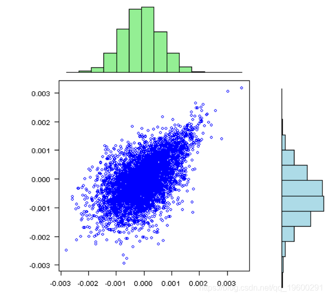
visualize.rets(fit.sim)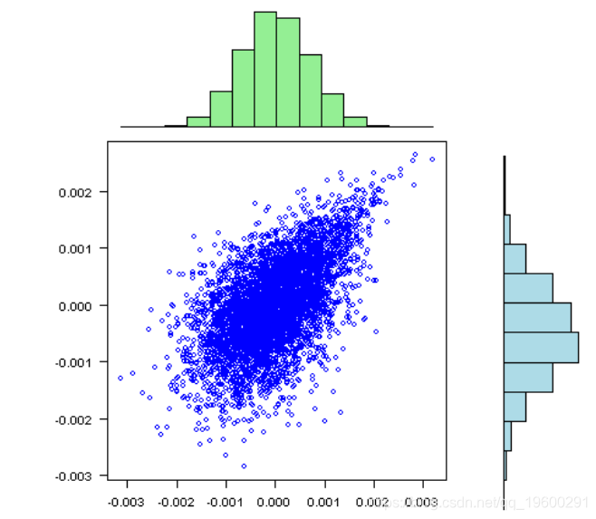
-
# qnorm(runif(10^8)) 和 rnorm(10^8) 是等价的
-
uniform.sim = rCopula(4800, gumbelCopula(gumbel@estimate, dim=n))
-
-
Actual Simulated
-
Correlation 57.13 57.14
-
Mean FB -0.31 -0.22
-
Mean YHOO -0.40 -0.56
-
StDev FB 1.24 1.24
-
StDev YHOO 1.23 1.21
FB
-
Two-sample Kolmogorov-Smirnov test
-
-
data: rets[, i] and fit.sim[i]
-
D = 0.7791, p-value = 0.5787
-
alternative hypothesis: two-sided
-
HO
-
Two-sample Kolmogorov-Smirnov test
-
-
data: rets[, i] and fit.sim[i]
-
D = 0.795, p-value = 0.5525
-
alternative hypothesis: two-sided
-

vis(rets)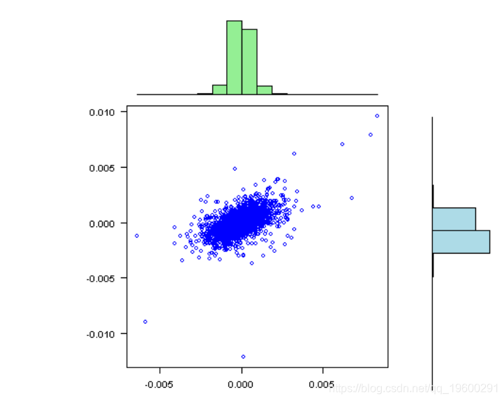
标准偏差相对于均值而言非常大,接近于零;因此,在某些情况下,我们很有可能获得不稳定的结果。

最受欢迎的见解
1.R语言基于ARMA-GARCH-VaR模型拟合和预测实证研究