R语言用逻辑回归、决策树和随机森林对信贷数据集进行分类预测

原文链接：http://tecdat.cn/?p=17950 

在本文中，我们使用了逻辑回归、决策树和随机森林模型来对信用数据集进行分类预测并比较了它们的性能。数据集是

credit=read.csv("german_credit.csv", header = TRUE, sep = ",")

看起来所有变量都是数字变量，但实际上，大多数都是因子变量，

1.  
   > str(credit)
2.  
   'data.frame': 1000 obs. of 21 variables:
3.  
   $ Creditability : int 1 1 1 1 1 1 1 1 1 1 ...
4.  
   $ Account.Balance : int 1 1 2 1 1 1 1 1 4 2 ...
5.  
   $ Duration : int 18 9 12 12 12 10 8 ...
6.  
   $ Purpose : int 2 0 9 0 0 0 0 0 3 3 ...

让我们将分类变量转换为因子变量，

1.  
   > F=c(1,2,4,5,7,8,9,10,11,12,13,15,16,17,18,19,20)
2.  
   > for(i in F) credit[,i]=as.factor(credit[,i])

现在让我们创建比例为1：2 的训练和测试数据集

1.  
   > i_test=sample(1:nrow(credit),size=333)
2.  
   > i_calibration=(1:nrow(credit))[-i_test]

我们可以拟合的第一个模型是对选定协变量的逻辑回归

1.  
   > LogisticModel <- glm(Creditability ~ Account.Balance + Payment.Status.of.Previous.Credit + Purpose +
2.  
   Length.of.current.employment +
3.  
   Sex...Marital.Status, family=binomia

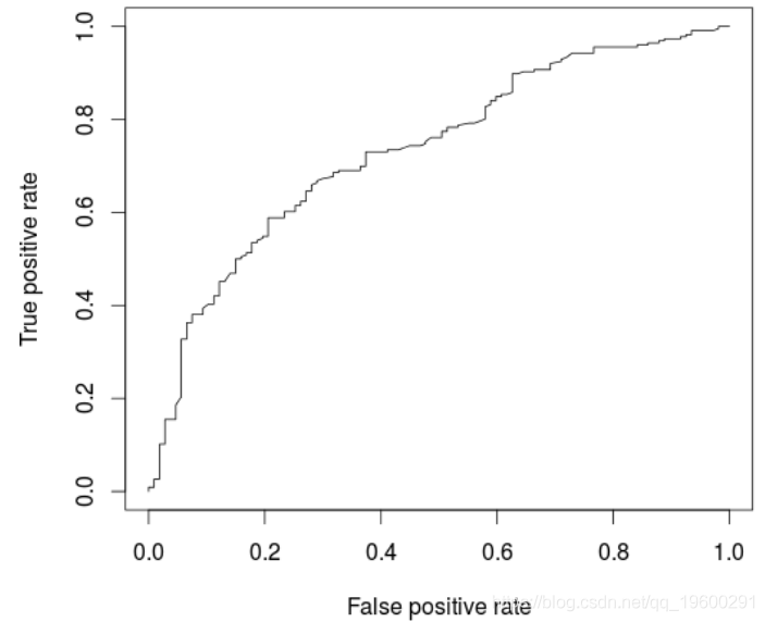
基于该模型，可以绘制ROC曲线并计算AUC（在新的验证数据集上）

1.  
    
2.  
   > AUCLog1=performance(pred, measure = "auc")@y.values[[1]]
3.  
   > cat("AUC: ",AUCLog1," ")
4.  
   AUC: 0.7340997

一种替代方法是考虑所有解释变量的逻辑回归

1.  
   glm(Creditability ~ .,
2.  
   + family=binomial,
3.  
   + data = credit[i_calibrat

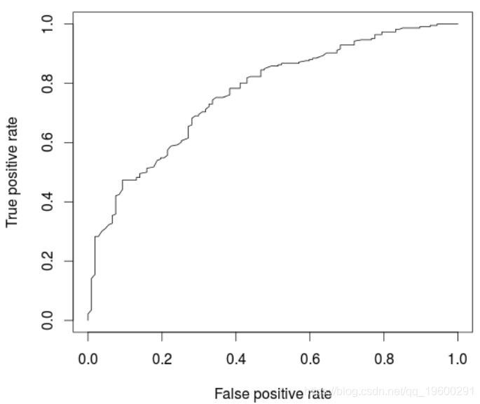
我们可能在这里过拟合，可以在ROC曲线上观察到

1.  
    
2.  
   > perf <- performance(pred, "tpr", "fpr
3.  
   > AUCLog2=performance(pred, measure = "auc")@y.values[[1]]
4.  
   > cat("AUC: ",AUCLog2," ")
5.  
   AUC: 0.7609792

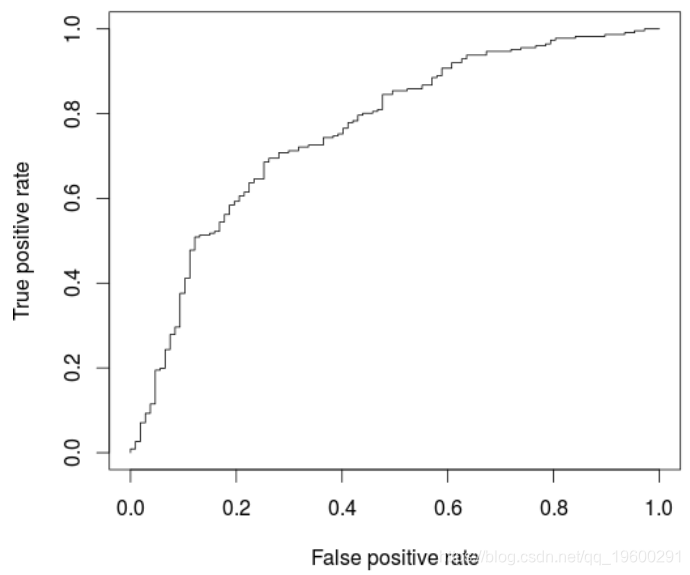
与以前的模型相比，此处略有改善，后者仅考虑了五个解释变量。

现在考虑回归树模型（在所有协变量上）

我们可以使用

> prp(ArbreModel,type=2,extra=1)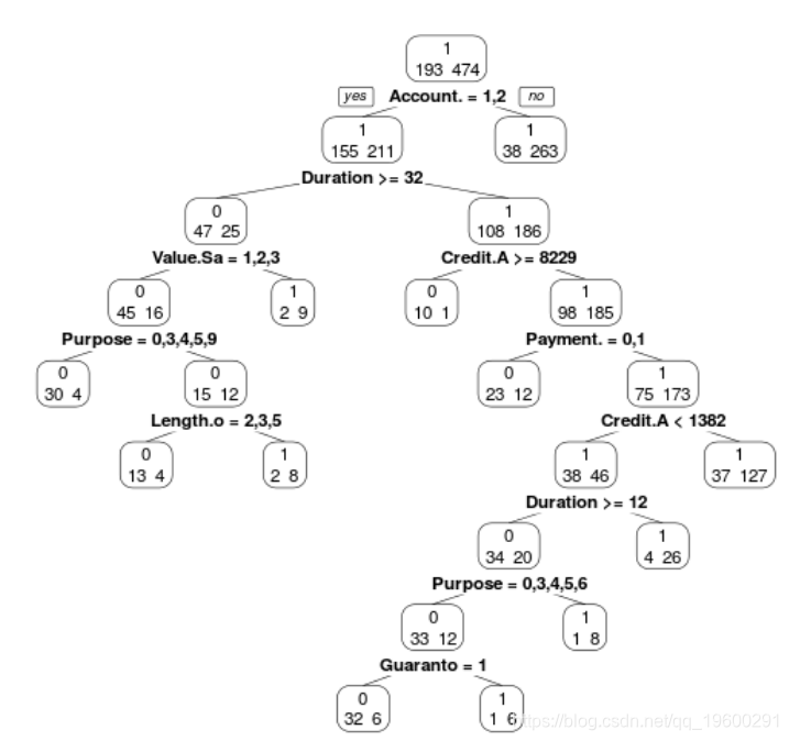

模型的ROC曲线为

1.  
   (pred, "tpr", "fpr")
2.  
   > plot(perf)
3.  
    
4.  
   > cat("AUC: ",AUCArbre," ")
5.  
   AUC: 0.7100323

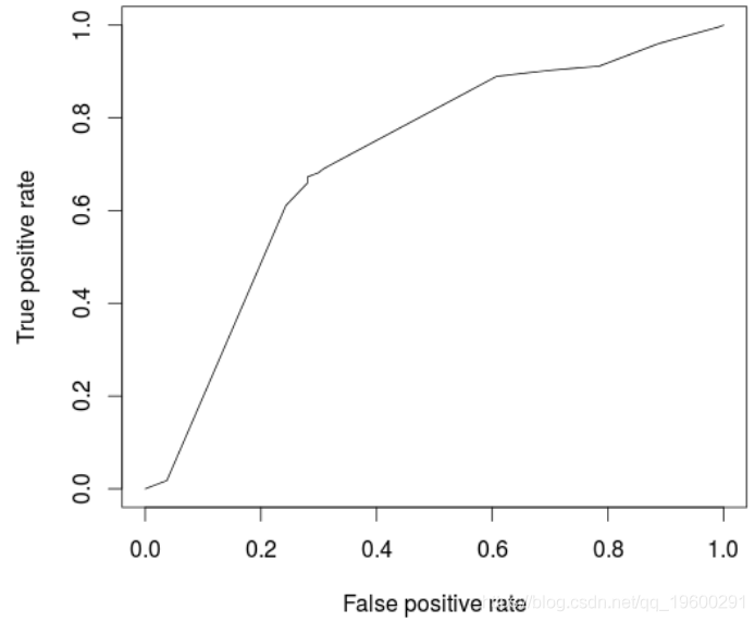
不出所料，与逻辑回归相比，模型性能较低。一个自然的想法是使用随机森林优化。

1.  
   > library(randomForest)
2.  
   > RF <- randomForest(Creditability ~ .,
3.  
   + data = credit[i_calibration,])
4.  
   > fitForet <- predict(RF,
5.  
    
6.  
   > cat("AUC: ",AUCRF," ")
7.  
   AUC: 0.7682367

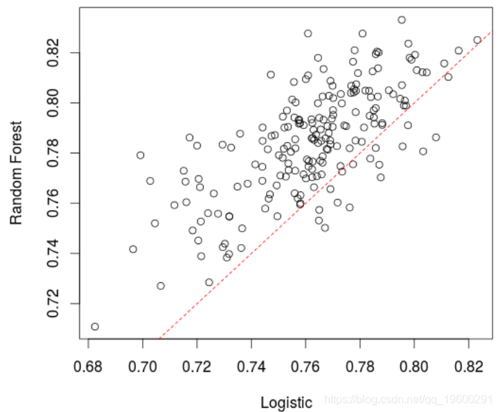
在这里，该模型（略）优于逻辑回归。实际上，如果我们创建很多训练/验证样本并比较AUC，平均而言，随机森林的表现要比逻辑回归好，

1.  
   > AUCfun=function(i){
2.  
   + set.seed(i)
3.  
   + i_test=sample(1:nrow(credit),size=333)
4.  
   + i_calibration=(1:nrow(credit))[-i_test]
5.  
    
6.  
    
7.  
   + summary(LogisticModel)
8.  
   + fitLog <- predict(LogisticModel,type="response",
9.  
   + newdata=credit[i_test,])
10.  
    + library(ROCR)
11.  
    + pred = prediction( fitLog, credit$Creditability[i_test])
12.  
     
13.  
    + RF <- randomForest(Creditability ~ .,
14.  
    + data = credit[i_calibration,])
15.  
     
16.  
     
17.  
    + pred = prediction( fitForet, credit$Creditability[i_test])
18.  
     
19.  
    + return(c(AUCLog2,AUCRF))
20.  
    + }
21.  
    > plot(t(A))

---

最受欢迎的见解

1.从决策树模型看员工为什么离职

2.R语言基于树的方法：决策树，随机森林

3.python中使用scikit-learn和pandas决策树

4.机器学习：在SAS中运行随机森林数据分析报告

5.R语言用随机森林和文本挖掘提高航空公司客户满意度

6.机器学习助推快时尚精准销售时间序列

7.用机器学习识别不断变化的股市状况——隐马尔可夫模型的应用

8.python机器学习：推荐系统实现（以矩阵分解来协同过滤）

9.python中用pytorch机器学习分类预测银行客户流失