原文链接:http://tecdat.cn/?p=17931
动量和马科维茨投资组合模型使 均值方差优化 组合成为可行的解决方案。通过建议并测试:
- 增加最大权重限制
- 增加目标波动率约束
来控制 均值方差最优化的解。
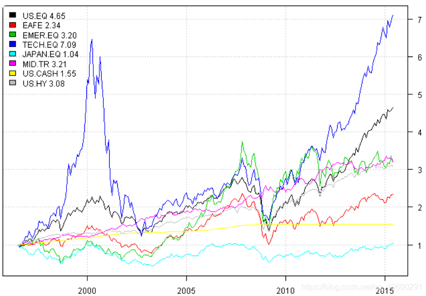
下面,我将查看8个资产的结果:
首先,让我们加载所有历史数据
-
#*****************************************************************
-
# 加载历史数据
-
-
#*****************************************************************
-
-
load.packages('quantmod')
-
-
# 加载保存的原始数据
-
#
-
load('raw.Rdata')
-
-
-
-
getSymbols.extra(N8.tickers, src = 'yahoo', from = '1970-01-01', env = data, raw.data =
-
for(i in data$symbolnames) data[[i]] = adjustOHLC(data[[i]]
-
接下来,让我们测试函数
-
#*****************************************************************
-
# 运行测试,每月数据
-
#*****************************************************************
-
-
plot(scale.one(data$prices))
-
prices = data$prices
-
-
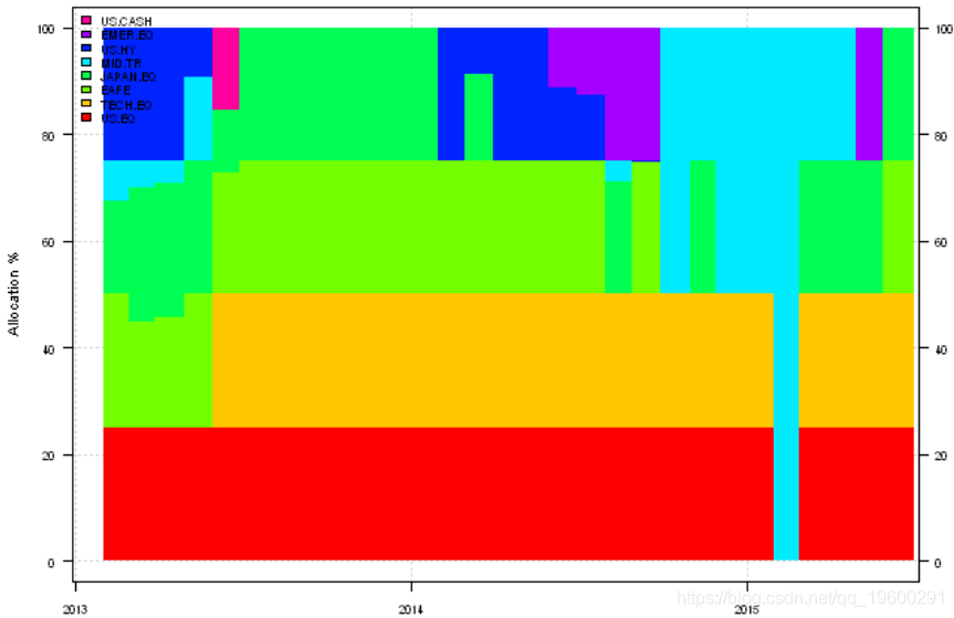
plotransition(res[[1]]['2013::'])
接下来,让我们创建一个基准并设置用于所有测试。
-
#*****************************************************************
-
# 建立基准
-
#*****************************************************************
-
models = list()
-
-
commission = list(cps = 0.01, fixed = 10.0, percentage = 0.0)
-
-
data$weight[] = NA
-
-
model = brun(data, clean.signal=T,
接下来,让我们获取权重,并使用它们来进行回测
-
#*****************************************************************
-
# 转换为模型结果
-
#*****************************************************************
-
CLA = list(weight = res[[1]], ret = res[[2]], equity = cumprod(1 + res[[2]]), type = "weight")
-
-
obj = list(weights = list(CLA = res[[1]]), period.ends
我们可以复制相同的结果
-
#*****************************************************************
-
#进行复制
-
#*****************************************************************
-
weight.limit = data.frame(last(pric
-
obj = portfoli(data$prices,
-
periodicity = 'months', lookback.len = 12, silent=T,
-
const.ub = weight.limit,urns,1) + colSums(last(hist.returns,3)) +
-
colSums(last(hist.returns,6)) + colSums(last(hist.returns,12))) / 22
-
ia
-
},
-
min.risk.fns = list(
-
)
-
-
另一个想法是使用Pierre Chretien的平均输入假设
-
#*****************************************************************
-
# 让我们使用Pierre的平均输入假设
-
#*****************************************************************
-
obj = portfolio(data$prices,
-
periodicity = 'months', lookback.len = 12, si
-
create.ia.fn = create.(c(1,3,6,12), 0),
-
min.risk.fns = list(
-
TRISK.AVG = target.risk.portfolio(target.r
-
)
-
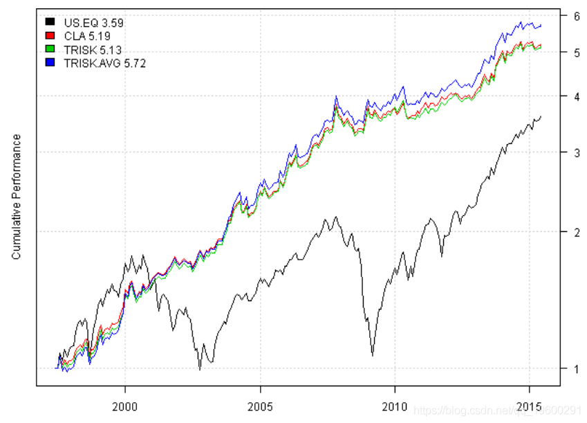
最后,我们准备看一下结果
-
#*****************************************************************
-
#进行回测
-
#*****************************************************************
-
-
plotb(models, plotX = T, log = 'y', Left
-
layout(1)
-
barplot(sapply(models, turnover, data)
使用平均输入假设会产生更好的结果。
我想应该注意的主要观点是:避免盲目使用优化。相反,您应该使解决方案更具有稳健性。

最受欢迎的见解
1.用机器学习识别不断变化的股市状况—隐马尔科夫模型(HMM)的应用