原文链接:http://tecdat.cn/?p=16881
灰色关联分析包括两个重要功能。
第一项功能:灰色关联度,与correlation系数相似,如果要评估某些单位,在使用此功能之前转置数据。第二个功能:灰色聚类,如层次聚类。
灰色关联度
灰色关联度有两种用法。该算法用于测量两个变量的相似性,就像`cor`一样。如果要评估某些单位,可以转置数据集。
*一种是检查两个变量的相关性,数据类型如下:
| 参考| v1 | v2 | v3 |
| ----------- |||| ---- | ---- |
| 1.2 | 1.8 | 0.9 | 8.4 |
| 0.11 | 0.3 | 0.5 | 0.2 |
| 1.3 | 0.7 | 0.12 | 0.98 |
| 1.9 | 1.09 | 2.8 | 0.99 |
reference:参考变量,reference和v1之间的灰色关联度...近似地测量reference和v1的相似度。
*另一个是评估某些单位的好坏。
| 单位| v1 | v2 | v3 |
| ----------- |||| ---- | ---- |
| 江苏| 1.8 | 0.9 | 8.4 |
| 浙江| 0.3 | 0.5 | 0.2 |
| 安徽 0.7 | 0.12 | 0.98 |
| 福建| 1.09 | 2.8 | 0.99 |
示例
-
-
##生成数据
-
-
#' economyCompare = data.frame(refer, liaoning, shandong, jiangsu, zhejiang, fujian, guangdong)
-
-
#
-
# 异常控制 #
-
if (any(is.na(df))) stop("'df' have NA" )
-
if (distingCoeff<0 | distingCoeff>1) stop("'distingCoeff' must be in range of [0,1]" )
-
-
-
-
-
diff = X #设置差学列矩阵空间
-
-
for (i in
-
mx = max(diff)
-
-
-
#计算关联系数#
-
relations = (mi+distingCoeff*mx) / (diff + distingCoeff*mx)
-
-
#计算关联度#
-
# 暂时简单处理, 等权
-
relDegree = rep(NA, nc)
-
for (i in 1:nc) {
-
relDegree[i] = mean(relations[,i]) # 等权
-
}
-
-
-
#排序: 按关联度大到小#
-
X_order = X[order(relDegree,
-
relDes = rep(NA, nc) #分配空间 关联关系描述(说明谁和谁的关联度)
-
X_names = names(X_o
-
names(relationalDegree) = relDes
-
-
-
if (cluster) {
-
-
greyRelDegree = GRA(economyC
-
-
-
# 得到差异率矩阵 #
-
grey_diff = matrix(0
-
-
grey_diff[i,j] = abs(rel
-
#得到距离矩阵#
-
grey_dist = matrix(0, nrow
-
iff[i,j]+grey_diff[j,i]
-
}
-
}
-
-
# 得到灰色相关系数矩阵 #
-
grey_dist_max = max(grey_dist)
-
grey_correl = matrix(0, nrow = nc, ncol = nc)
-
for (i in 1:nc) {
-
for (j in 1:nc) {
-
grey_correl[i,j] = 1 - grey_dist[i,j] / grey_dist_max
-
}
-
}
-
-
-
-
d = as.dist(1-grey_correl) # 得到无对角线的下三角矩阵(数值意义反向了, 值越小表示越相关 )
-
# 主对角线其实表示了各个对象的相近程度, 画图的时候, 相近的对象放在一起
-
-
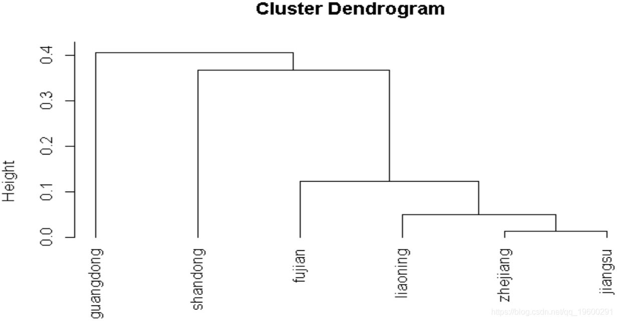
hc = hclust(d, method = clusterMethod) # 系统聚类(分层聚类)函数, single: 单一连接(最短距离法/最近邻)
-
# hc$height, 是上面矩阵的对角元素升序
-
# hc$order, 层次树图上横轴个体序号
-
plot(hc,hang=-1) #hang: 设置标签悬挂位置
-
-
}
-
-
#输出#
-
-
if (cluster) {
-
lst = list(relationalDegree=relationalDegree,
-
-
return(lst)
-
-
}
-
```
-
-
-
-
```{r}
-
## 生成数据
-
rownames(economyCompare) = c("indGV", "indVA", "profit", "incomeTax")
-
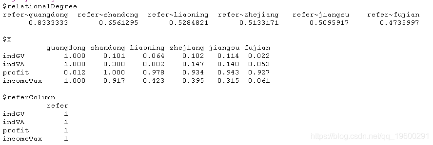
## 灰色关联度
-
greyRelDegree = greya(economyCompare)
-
greyRelDegree
-
```
-
-
-
灰色关联度
灰色聚类,如层次聚类
-
-
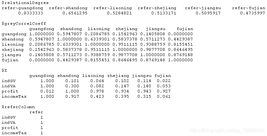
## 灰色聚类
-
-
greya(economyCompare, cluster = T)
-

最受欢迎的见解
3.R语言对用电负荷时间序列数据进行K-medoids聚类建模和GAM回归
5.Python Monte Carlo K-Means聚类实战