原文链接:http://tecdat.cn/?p=5453
变量选择方法
所有可能的回归
model <- lm(mpg ~ disp + hp + wt + qsec, data = mtcars)
ols_all_subset(model)

## # A tibble: 15 x 6
##    Index     N      Predictors `R-Square` `Adj. R-Square` `Mallow's Cp`
##
##  1     1     1              wt    0.75283         0.74459      12.48094
##  2     2     1            disp    0.71834         0.70895      18.12961
##  3     3     1              hp    0.60244         0.58919      37.11264
##  4     4     1            qsec    0.17530         0.14781     107.06962
##  5     5     2           hp wt    0.82679         0.81484       2.36900
##  6     6     2         wt qsec    0.82642         0.81444       2.42949
##  7     7     2         disp wt    0.78093         0.76582       9.87910
##  8     8     2         disp hp    0.74824         0.73088      15.23312
##  9     9     2       disp qsec    0.72156         0.70236      19.60281
## 10    10     2         hp qsec    0.63688         0.61183      33.47215
## 11    11     3      hp wt qsec    0.83477         0.81706       3.06167
## 12    12     3      disp hp wt    0.82684         0.80828       4.36070
## 13    13     3    disp wt qsec    0.82642         0.80782       4.42934
## 14    14     3    disp hp qsec    0.75420         0.72786      16.25779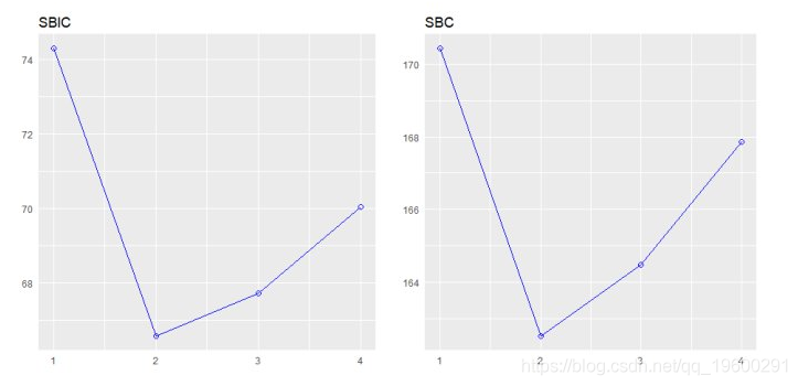
## 15 15 4 disp hp wt qsec 0.83514 0.81072 5.00000该plot方法显示了所有可能的回归方法的拟合 。
model <- lm(mpg ~ disp + hp + wt + qsec, data = mtcars)
k <- ols_all_subset(model)
plot(k)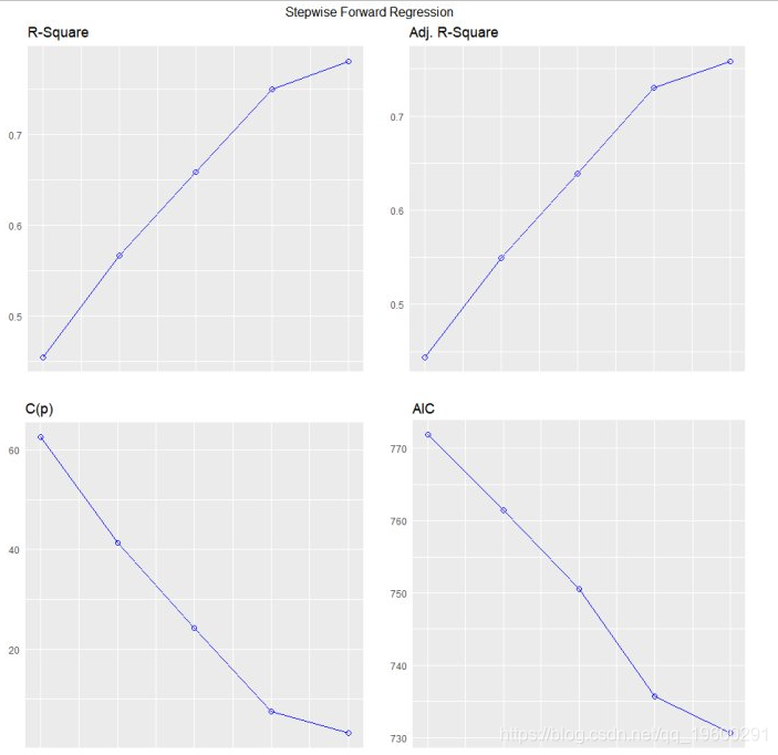
![]()
![]()
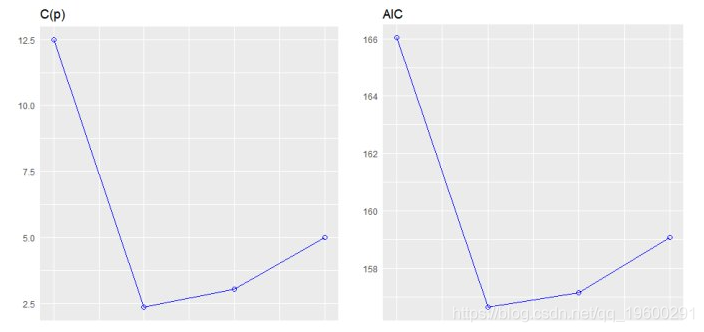
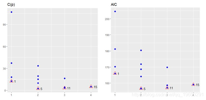
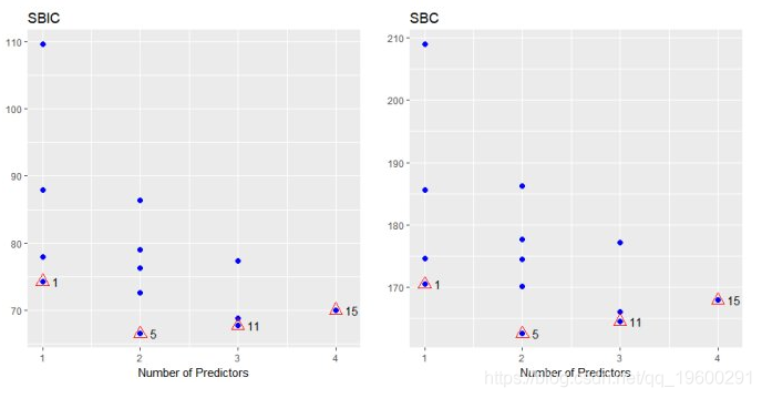
最佳子集回归
选择在满足一些明确的客观标准时做得最好的预测变量的子集,例如具有最大R2值或最小MSE, Cp或AIC。
model <- lm(mpg ~ disp + hp + wt + qsec, data = mtcars)
ols_best_subset(model)

##    Best Subsets Regression
## ------------------------------
## Model Index    Predictors
## ------------------------------
##      1         wt
##      2         hp wt
##      3         hp wt qsec
##      4         disp hp wt qsec
## ------------------------------
##
##                                                   Subsets Regression Summary
## -------------------------------------------------------------------------------------------------------------------------------
##                        Adj.        Pred
## Model    R-Square    R-Square    R-Square     C(p)        AIC        SBIC        SBC        MSEP      FPE       HSP       APC
## -------------------------------------------------------------------------------------------------------------------------------
##   1        0.7528      0.7446      0.7087    12.4809    166.0294    74.2916    170.4266    9.8972    9.8572    0.3199    0.2801
##   2        0.8268      0.8148      0.7811     2.3690    156.6523    66.5755    162.5153    7.4314    7.3563    0.2402    0.2091
##   3        0.8348      0.8171       0.782     3.0617    157.1426    67.7238    164.4713    7.6140    7.4756    0.2461    0.2124
##   4        0.8351      0.8107       0.771     5.0000    159.0696    70.0408    167.8640    8.1810    7.9497    0.2644    0.2259
## -------------------------------------------------------------------------------------------------------------------------------
## AIC: Akaike Information Criteria
##  SBIC: Sawa's Bayesian Information Criteria
##  SBC: Schwarz Bayesian Criteria
##  MSEP: Estimated error of prediction, assuming multivariate normality
##  FPE: Final Prediction Error
##  HSP: Hocking's Sp
##  APC: Amemiya Prediction Criteria
plot
model <- lm(mpg ~ disp + hp + wt + qsec, data = mtcars)
k <- ols_best_subset(model)
plot(k)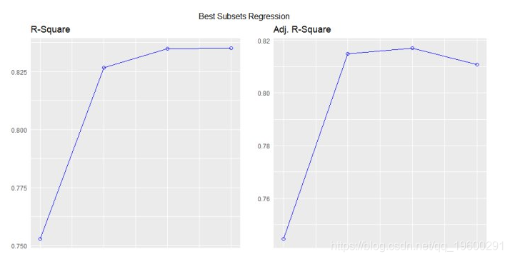
![]()
![]()
![]()
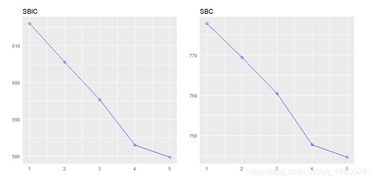
逐步前进回归
从一组候选预测变量中建立回归模型,方法是逐步输入基于p值的预测变量,直到没有变量进入变量。该模型应该包括所有的候选预测变量。如果细节设置为TRUE,则显示每个步骤。
变量选择
# stepwise forward regression
model <- lm(y ~ ., data = surgical)
ols_step_forward(model)

## We are selecting variables based on p value...

## 1 variable(s) added....

## 1 variable(s) added...
## 1 variable(s) added...
## 1 variable(s) added...
## 1 variable(s) added...

## No more variables satisfy the condition of penter: 0.3

## Forward Selection Method
##
## Candidate Terms:
##
## 1 . bcs
## 2 . pindex
## 3 . enzyme_test
## 4 . liver_test
## 5 . age
## 6 . gender
## 7 . alc_mod
## 8 . alc_heavy
##
## ------------------------------------------------------------------------------
##                               Selection Summary
## ------------------------------------------------------------------------------
##         Variable                     Adj.
## Step      Entered      R-Square    R-Square     C(p)        AIC         RMSE
## ------------------------------------------------------------------------------
##    1    liver_test       0.4545      0.4440    62.5119    771.8753    296.2992
##    2    alc_heavy        0.5667      0.5498    41.3681    761.4394    266.6484
##    3    enzyme_test      0.6590      0.6385    24.3379    750.5089    238.9145
##    4    pindex           0.7501      0.7297     7.5373    735.7146    206.5835
##    5    bcs              0.7809      0.7581     3.1925    730.6204    195.4544
## ------------------------------------------------------------------------------


model <- lm(y ~ ., data = surgical)
k <- ols_step_forward(model)

## We are selecting variables based on p value...

## 1 variable(s) added....

## 1 variable(s) added...
## 1 variable(s) added...
## 1 variable(s) added...
## 1 variable(s) added...

## No more variables satisfy the condition of penter: 0.3

plot(k)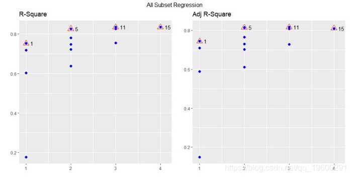
![]()
![]()
![]()