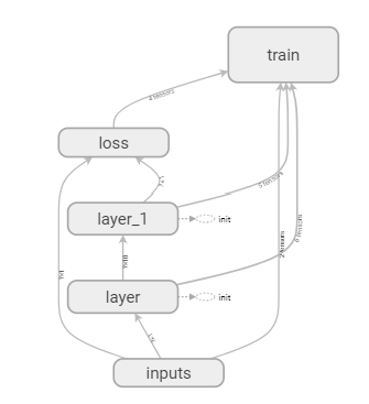
1. 使用 with tf.name_scope('layer') 加标签
def add_layer(inputs, in_size, out_size, activation_function=None):
    with tf.name_scope('layer'):
        with tf.name_scope('weights'):
            Weight = tf.Variable(tf.random_normal([in_size, out_size]), name='W')  # 初始权重随机
        with tf.name_scope('biases'):
            biases = tf.Variable(tf.zeros([1, out_size]) + 0.1, name='b')  # biases推荐不为0,所以需要加上0.1
        with tf.name_scope('Wx_plus_b'):
            Wx_plus_b = tf.add(tf.matmul(inputs, Weight), biases)  # 激活前
        if activation_function is None:
            outputs = Wx_plus_b
        else:
            outputs = activation_function(Wx_plus_b)
        return outputs
2. pycharm terminal 中进入project目录
输入 tensorboard --logdir=logs
将得到的网址 http://DESKTOP-V7I30OQ:6006 输入浏览器,即可得到
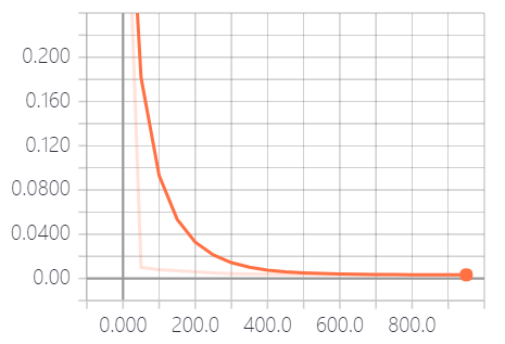
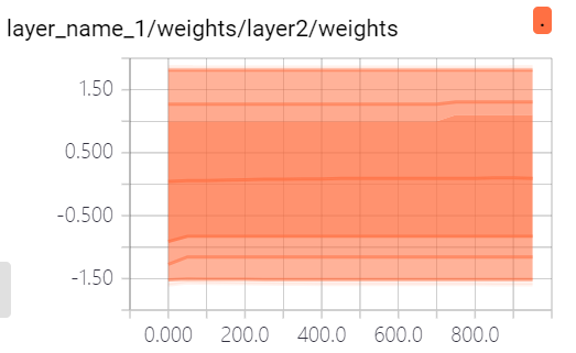
3. 查看weight、biases、loss
tf.summary.histogram(layer_name+'/weights', Weight)
tf.summary.histogram(layer_name + '/biases', biases)
tf.summary.scalar('loss', loss)
merged = tf.summary.merge_all()  # 打包
result = sess.run(merged, feed_dict={xs: x_data, ys: y_data})
writer.add_summary(result, i)  # 每i步画一个点
4. 参考代码
import tensorflow as tf
import numpy as np
import matplotlib.pyplot as plt


def add_layer(inputs, in_size, out_size, n_layer, activation_function=None):
    layer_name = 'layer%s' % n_layer
    with tf.name_scope('layer_name'):
        with tf.name_scope('weights'):
            Weight = tf.Variable(tf.random_normal([in_size, out_size]), name='W')  # 初始权重随机
            tf.summary.histogram(layer_name+'/weights', Weight)
        with tf.name_scope('biases'):
            biases = tf.Variable(tf.zeros([1, out_size]) + 0.1, name='b')  # biases推荐不为0,所以需要加上0.1
            tf.summary.histogram(layer_name + '/biases', biases)
        with tf.name_scope('Wx_plus_b'):
            Wx_plus_b = tf.add(tf.matmul(inputs, Weight), biases)  # 激活前
        if activation_function is None:
            outputs = Wx_plus_b
        else:
            outputs = activation_function(Wx_plus_b)
        tf.summary.histogram(layer_name + '/outputs', outputs)
        return outputs


# 数据准备
x_data = np.linspace(-1, 1, 300)[:, np.newaxis]   # 生成[-1,1]之间的300个数,组成300行的一个数组
noise = np.random.normal(0, 0.05, x_data.shape)  # mean = 0;std = 0.05; 格式:x_data
y_data = np.square(x_data) - 0.5 + noise  # y = x^2 - 0.5
with tf.name_scope('inputs'):
    xs = tf.placeholder(tf.float32, [None, 1], name='x_input')  # None表示sample数量任意
    ys = tf.placeholder(tf.float32, [None, 1], name='y_input')

# 搭建神经网络
# 由于输入一维,输出一维,所以我们定义的神经网络为输入层一个神经元,输出层一个神经元,中间隐藏层10个神经元
l1 = add_layer(xs, 1, 10, n_layer=1, activation_function=tf.nn.relu)  # 隐藏层
prediction = add_layer(l1, 10, 1, n_layer=2, activation_function=None)  # 输出层
# 计算损失函数
with tf.name_scope('loss'):
    loss = tf.reduce_mean(tf.reduce_sum(tf.square(ys - prediction), reduction_indices=[1]))   # 距离平方求和求平均,reduction_indices表示数据处理的维度
    tf.summary.scalar('loss', loss)
# 训练
with tf.name_scope('train'):
    train_step = tf.train.GradientDescentOptimizer(0.1).minimize(loss)  # learning rate = 0.1

# 初始化
init = tf.initialize_all_variables()  # 初始化所有变量
sess = tf.Session()
merged = tf.summary.merge_all()
writer = tf.summary.FileWriter("logs/", sess.graph)
sess.run(init)

# 可视化输出
fig = plt.figure()
ax = fig.add_subplot(1, 1, 1)
ax.scatter(x_data, y_data)
plt.ion()  # 保证连续输出
for i in range(1000):
    sess.run(train_step, feed_dict={xs: x_data, ys: y_data})
    if i % 50 == 0:  # 每50个数据输出一次
        try:  # 为了避免第一次remove时报错
            ax.lines.remove(lines[0])
        except Exception:
            pass
        prediction_value = sess.run(prediction, feed_dict={xs: x_data})
        lines = ax.plot(x_data, prediction_value, 'r-', lw=5)
        plt.pause(0.1)  # 暂停0.1秒
        result = sess.run(merged, feed_dict={xs: x_data, ys: y_data})
        writer.add_summary(result, i)  # 每i步画一个点