Chapter 5 Image Restoration and Reconstruction 图像复原与重建
5.1 A Model of the Image Defradation/Restoration Process 图像退化/复原过程的模型
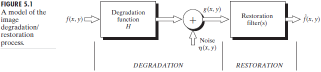
As Fig.5.1 shows,the degradation process is modeled as a degradation function (退化函数) with an additive noise term (加性噪声) ,operates on an input image \(f(x,y)\) to produce a degraded image \(g(x,y)\).Given \(g(x,y)\) ,some knowledge about the degradation function and the additive noise term \(\eta(x,y)\),the objective of restoration is to obtain an estimate \(\hat{f}(x,y)\)
通过退化后的图像\(g(x,y)\)以及退化函数和噪声获得原始图像的一个估计。
If H is a linear,position-invariant process,then the degrade image is given in the spatial domain by
write the model in an equivalent frequency domain representation(use Fourier Transform):
乘性噪声通过取对数的方式可以转换为加性噪声,故主要分析加性噪声的相关特性。
5.2 Noise Models 噪声模型
5.2.1 Spatial and Frequency Properties of Noise 噪声的空间和频率特性
white noise(白噪声),a random signal with a constant power spectral density 功率谱密度为常数的随机信号。理想的白噪声拥有无限大的带宽,实际中,我们常常将有限带宽的平整信号视为白噪声。
5.2.2 Some Important Noise Probability Density Functions 噪声概率密度函数
The spatial noise descriptor with which we shall be concerned is the statistical behavior of the intensity values in the noise component of the model in Fig.5.1.These may be considered random variables,characterized by a probability density function(PDF).
考虑噪声分量的灰度值统计特性(由概率密度函数PDF表征的随机变量)
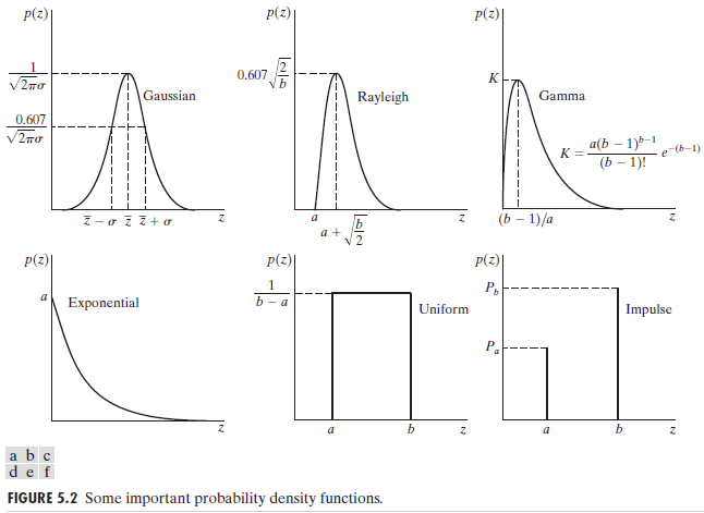
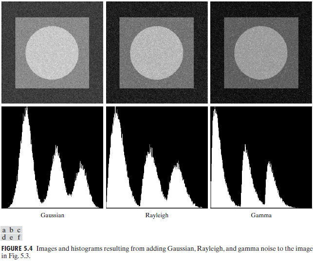
Gaussian noise 高斯噪声
also called normal noise (正态噪声),with mathematical tractability (数学上的易处理性)
The PDF of a Gaussian random variable,z,is given by
$$ p(z) = \frac{1}{\sqrt{2\pi}\sigma}e{-(z-\bar{z})2/{2\sigma^2}} $$
where \(z\) represents intensity,\(\bar{z}\) is the mean(average) value of \(z\), and \(\sigma\) is its standard deviation.The standard deviation squard,\(\sigma^2\),is called the variance of z.
\(z\) 表示灰度值, \(\bar{z}\)表示\(z\)的平均值, \(\sigma\)表示\(z\)的标准差, 标准差的平方\(\sigma^2\)称为\(z\)的方差。
Rayleigh noise 瑞利噪声
The PDF of Rayleigh noise is given by
The mean and variance of this density are given by
Erlang(gamma) noise 爱尔兰(伽马)噪声
The PDF of Gamma noise is given by
The mean and variance of this density are given by
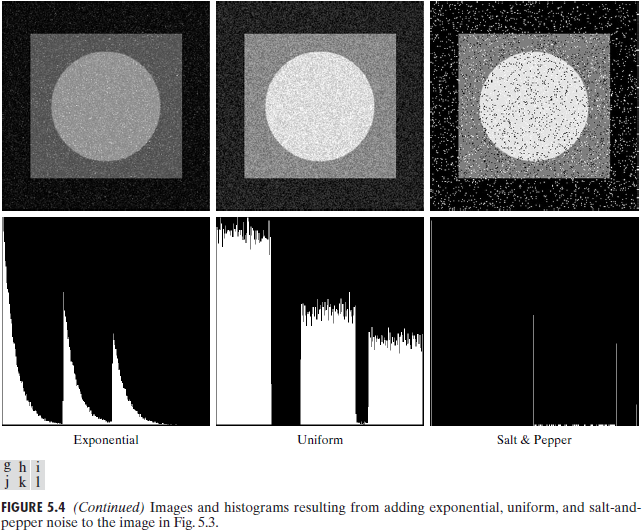
Exponential noise 指数噪声
The PDF of exponential noise is given by
where $ a > 0 $. The mean and variance of this density function are
Uniform noise 均匀噪声
The PDF of uniform noise is given by
The mean and variance of this density function are
Impulse (salt-and-pepper) noise 椒盐噪声
The PDF of exponential noise is given by
5.2.3 Periodic Noise 周期噪声
Periodic noise in an image arises typically from electrical or electromechanical interference during image acquisition.As discussed in Section 5.4,periodic noise can be reduced significantly via frequency domain filtering.
一幅图像中的周期噪声是在图像获取期间由电力或机电干扰产生的。周期噪声可以通过频率域滤波来显著减少。具体讨论见5.4节。
5.2.4 Estimation of Noise Parameters 噪声参数的估计
estimate the parameters of the PDF from small patches of reasonably constant background intensity.根据有着合理恒定灰度值的一小部分来估计PDF的参数。
考虑由S表示的一个子图像,并令\(p_s(z_i),i=0,1,2,...,L-1\)表示S中像素灰度的概率估计(归一化直方图值),其中L是整个图像中可能的灰度值(例如,对于8比特图像,L为256)。S的均值和方差。计算如下
5.3 Restoration in the Presence of Noise Only-Spatial Filtering 只存在噪声的复原-空间滤波
When the only degradation present in than image is noise,当图像中只有噪声引起的退化(忽略退化函数)时,we have
假设\(\hat{f}(x,u=y)\)为对图像的估计,则\(|\hat{f}(x,y)-g(x,y)|^2\)应该尽可能与已知的噪声分布一致,由此得出合理的估计值。
5.6 Estimating the Degradation Function 估计退化函数
5.6.1 Estimation by Image Observation 图像观察估计
根据$ g(x,y) = f(x,y) * h(x,y) + \eta(x,y) $,暂时忽略噪声,对该式作Fourier Transform,得到: $ G(u,v) = F(u,v) H(u,v) $ 故有 $$ H(u,v) = \frac{G(u,v)}{F(u,v)} $$
5.6.2 Estimation by Experimentation 试验估计
通过试验,找到与获取退化图像设备相似的装置,从而得到一个准确的退化估计。
根据$ g(x,y) = f(x,y) * h(x,y) \(,(忽略噪声),当\)f(x,y)\(为一个冲激函数\)\delta(x,y)\(时,卷积得到的\)g(x,y)\(就是\)h(x,y)$。
使用相同的系统对一个冲激(小亮点)成像,得到退化的冲激响应。
5.6.3 Estimation by Modeling 建模估计
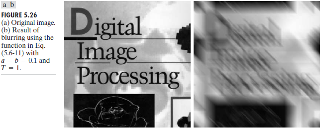
1、Turbulence (湍流模型),该模型通用形式为:
上式经Fourier Transform,得到
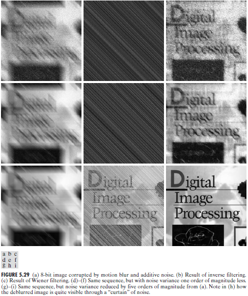
5.7 Inverse Filtering 逆滤波
通过退化图形的傅里叶变换 \(G(u,v)\) 与退化函数 \(H(u,v)\) 之比来计算原始图像的傅里叶变换的估计 \(\hat{F}(x,y)\) ,即
又有 \(G(u,v) = H(u,v)F(u,v) + N(u,v)\) ,代入上式,有
因为 \(N(u,v)\) 未知,所以即使知道退化函数,也并不能准确的复原图像。另外,如果退化函数是零或者非常小的值,则分式项值会非常大,很容易支配估计值 \(\hat{F}(u,v)\)。因此,直接逆滤波的性能是很差的,下面提到的维纳滤波器就是很好的改进方法。
5.8 Minimum Mean Square Error (Wiener) Filtering 最小均方差(维纳)滤波
该方法建立在图像和噪声都是随机变量的基础上,目标是找到未污染图像 \(f\) 的一个估计 \(\hat{f}\) ,使它们之间的均方误差最小。这种误差度量由下式给出
其中,\(E\{\cdot\}\)是参数的期望值。该误差函数的最小值在频率域中由如下表达式给出(最常用的近似式)
直接逆滤波和维纳滤波效果对比