一、单变量线性回归:
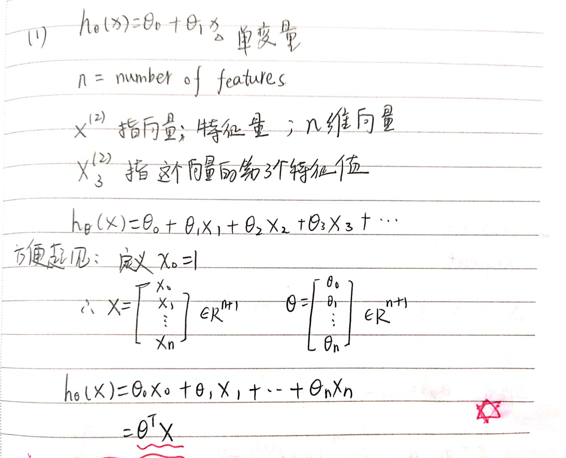
m训练样本,x输入变量特征(单变量特征只有一个),y输出变量即预测。如何用m个,特征为x的训练样本,来得到预测值?

假设函数:![]()
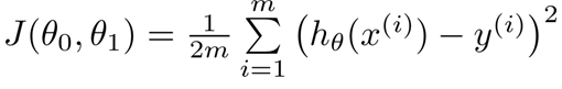
代价函数:
优化目标:使用梯度下降法优化θ值来最小化代价函数J。
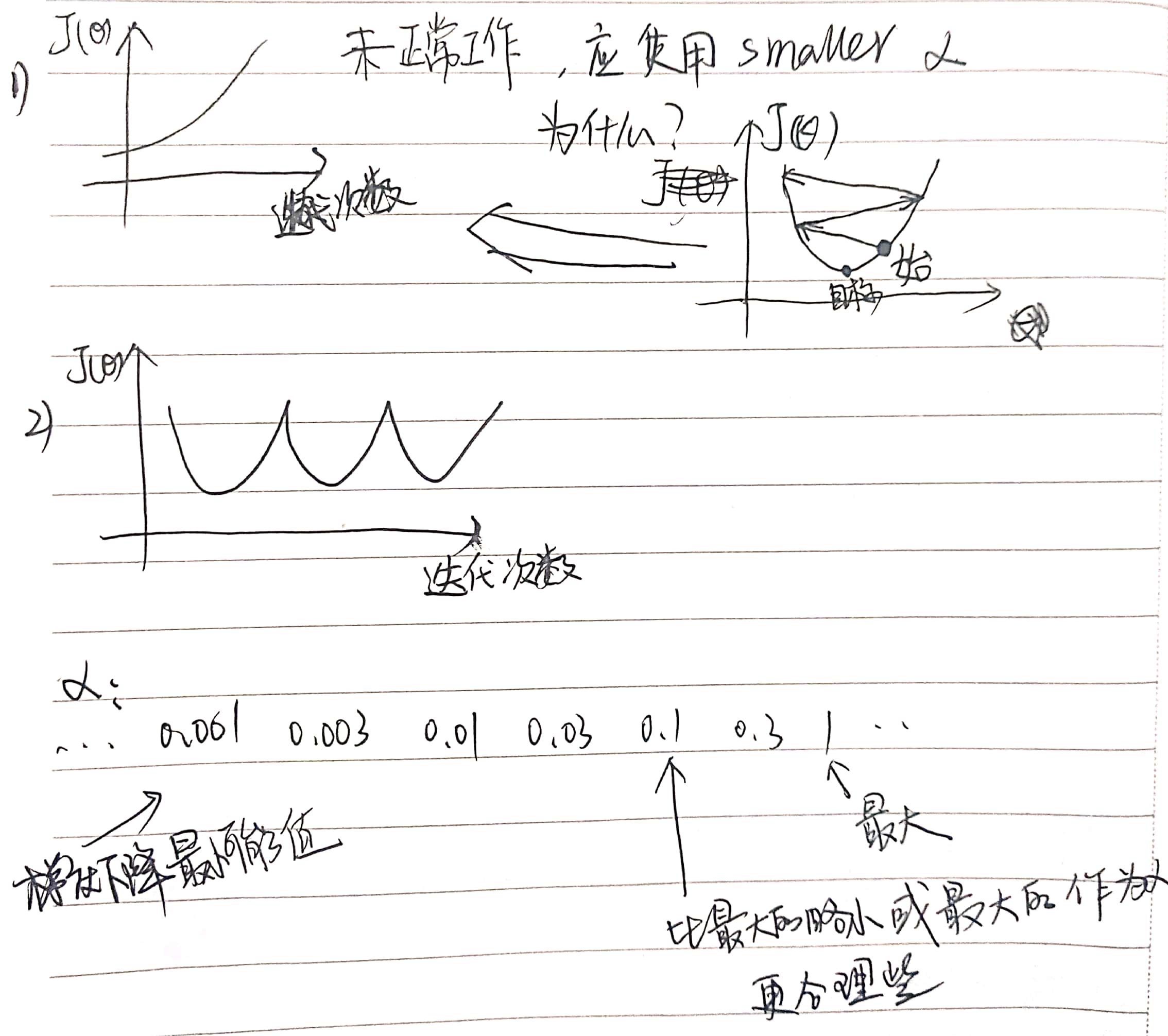
梯度是一个矢量,指其方向上的方向导数最大,即增长最快。
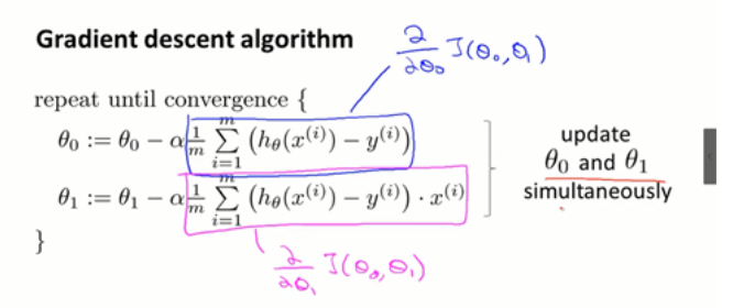
梯度下降法算法思想:
1) 初始化θ值,通常设为[0;0];
2) 不断改变θ大小来改变代价函数J,收敛至局部最小值。
注:θ的初始值不同最后得到的局部最优解也不同。参考图1-蒙着眼睛下山问题。
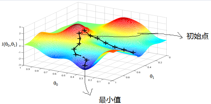
图1-蒙着眼睛下山

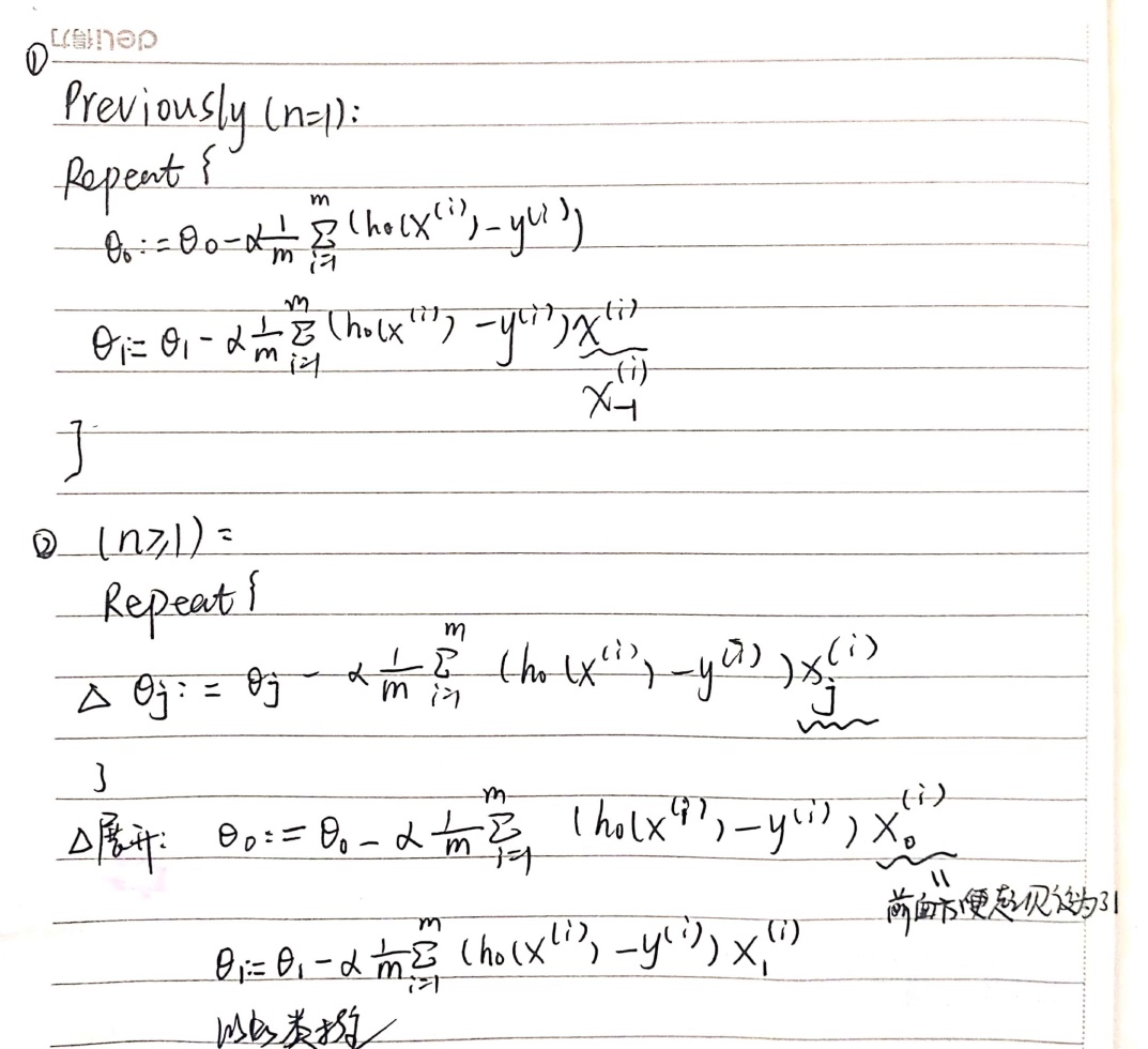
二、多变量线性回归:
单变量与多变量线性回归的梯度下降算法:
三、梯度下降法
1.特征缩放:
通常进行均值归一化:X1 =(X1 –均值)/ (max – min),使X1属于(-3,3)或者(-0.33,0.33)。其中max-min值不一定,只要值与其相近就可以,目的在于缩放。
2. α学习率
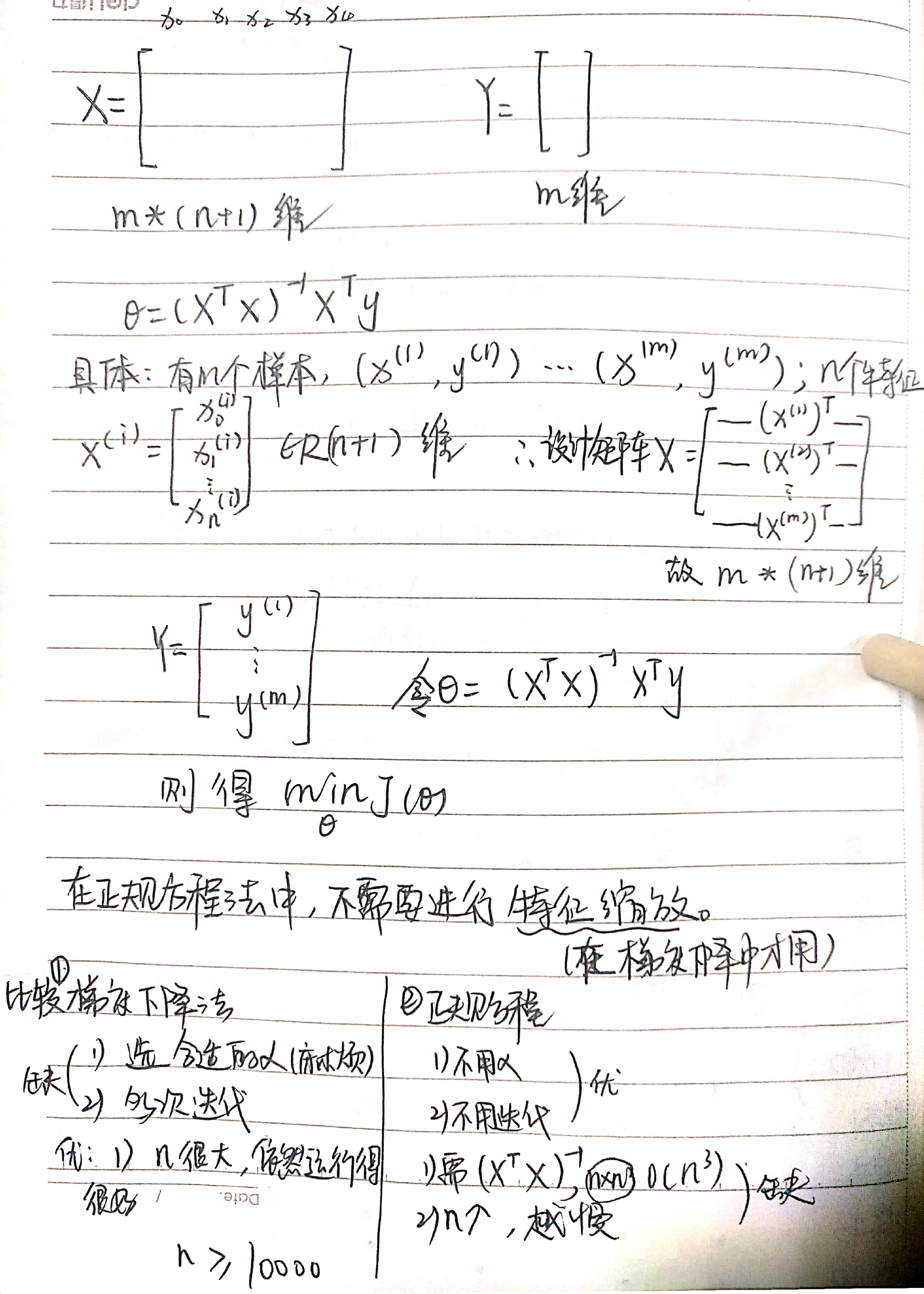
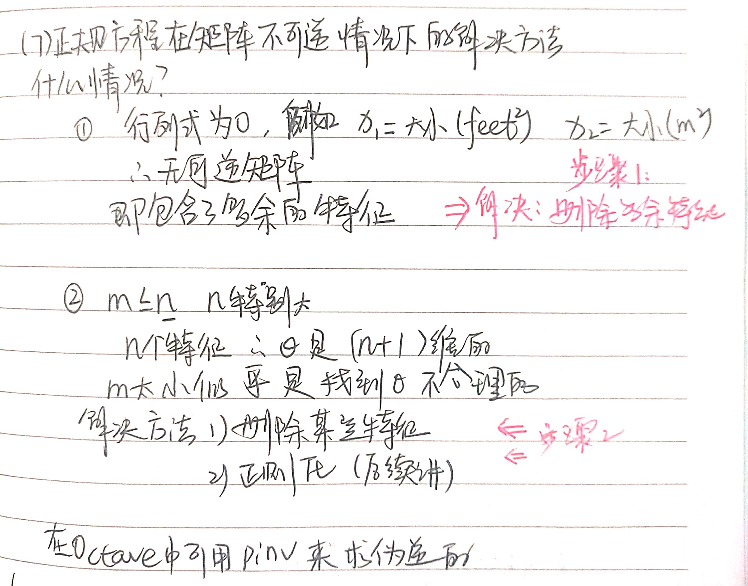
四、正规方程
区别于上述迭代方法(梯度下降)的直接方法。
五、第一次编程作业
1.单变量
(1).computeCost.m
完成对代价函数——![]() 的代码化。
的代码化。
function J = computeCost(X, y, theta)
%COMPUTECOST Compute cost for linear regression
%   J = COMPUTECOST(X, y, theta) computes the cost of using theta as the
%   parameter for linear regression to fit the data points in X and y

% Initialize some useful values
m = length(y); % number of training examples

% You need to return the following variables correctly
J = 0;

% ====================== YOUR CODE HERE ======================
% Instructions: Compute the cost of a particular choice of theta
%               You should set J to the cost.
M = (X*theta-y).^2;
J = sum(M(:))/m*0.5;
% =========================================================================

end
(2).gradientDescent.m
利用上述公式在for循环里实现梯度下降。
function [theta, J_history] = gradientDescent(X, y, theta, alpha, num_iters)
%GRADIENTDESCENT Performs gradient descent to learn theta
%   theta = GRADIENTDESCENT(X, y, theta, alpha, num_iters) updates theta by
%   taking num_iters gradient steps with learning rate alpha

% Initialize some useful values
m = length(y); % number of training examples
J_history = zeros(num_iters, 1);

for iter = 1:num_iters
   temp0 = theta(1)-sum((X*theta-y),1)/m*alpha
   temp1 = theta(2)-(X(:,2))'*(X*theta-y)/m*alpha
   theta(1) = temp0
   theta(2) = temp1

    % ====================== YOUR CODE HERE ======================
    % Instructions: Perform a single gradient step on the parameter vector
    %               theta.
    %
    % Hint: While debugging, it can be useful to print out the values
    %       of the cost function (computeCost) and gradient here.
    %
    % ============================================================

    % Save the cost J in every iteration
    J_history(iter) = computeCost(X, y, theta);
end
end
注:下面是错误的,因为进行梯度下降的时候是同时更新θ值。如果采用下面表达,更新θ2时,theta已经改变,破坏了同时更新。
theta(1)= theta(1)-sum((X*theta-y),1)/m*alpha
theta(2)= theta(2)-(X(:,2))'*(X*theta-y)/m*alpha
2.多变量
(1)FeatureNormalize.m
特征缩放,进行均值归一化
mu = mean(X,1);
sigma = std(X);
X_norm = (X_norm - mu)./sigma;
(2)computeCostMulti.m
代价函数与单变量一样
(3)gradientDescentMulti.m
与单变量不同,对θ矢量化
for iter = 1:num_iters
    for i = 1:size(X,2)
        temp(i,1) = theta(i)-(X(:,i))'*(X*theta-y)/m*alpha;
    end
    theta = temp;
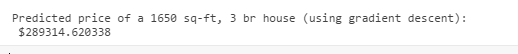
(4)预测价格
price = [1 ([1650 3]-mu)./sigma]*theta;
上述进行了特征缩放,故例子中的两个特征也须进行特征缩放。该方法预测结果如下:
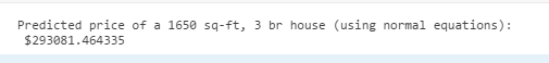
3.正规方程
normalEqn.m
function [theta] = normalEqn(X, y)
%NORMALEQN Computes the closed-form solution to linear regression
%   NORMALEQN(X,y) computes the closed-form solution to linear
%   regression using the normal equations.

theta = zeros(size(X, 2), 1);

% ====================== YOUR CODE HERE ======================
% Instructions: Complete the code to compute the closed form solution
%               to linear regression and put the result in theta.
%

% ---------------------- Sample Solution ----------------------

theta = pinv((X'*X))*X'*y;

% -------------------------------------------------------------


% ============================================================

end
正规方程中没有进行特征缩放,故预测价格代码如下。
price = [1 1650 3]*theta;
该方法预测结果如下: