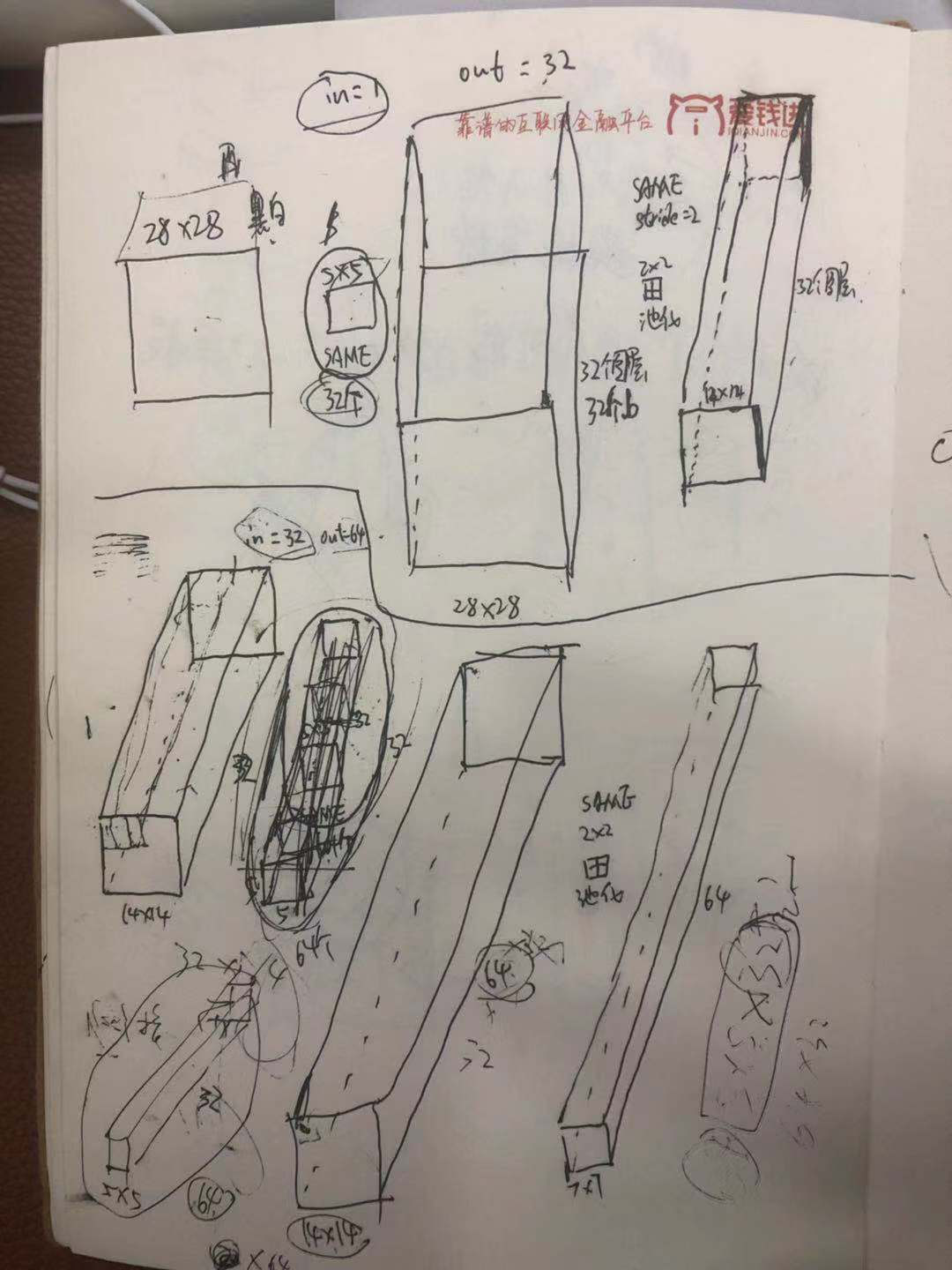
#!/usr/bin/env python
# -*- coding: utf-8 -*-
# @Time    : 2018/3/30 上午8:26
# @Author  : ruina.sun
# @Software: PyCharm Community Edition

import tensorflow as tf
import numpy as np
import matplotlib.pyplot as plt
from tensorflow.examples.tutorials.mnist import input_data
import os

pro_path = os.path.abspath('..')
# 样本个数是位置权值参数个数的5-30倍
# receptive field 感受野,猫看球视觉实验,部分视觉中枢的神经元是亮的,-->局部感受野。
# convolution (卷积)-->划窗,点乘求和
# pooling (池化)-->划窗,取max/mean值
# padding (填充)卷积和池化都存在窗格不够的情况,都需要padding处理方式。
#          步长为(1,1)的话:same-padding保留边缘信息,可能会补零以得到和原来平面一样大小,
#                         valid-padding有可能缺失边缘信息,不补零可能会得到比原来平面小的平面。
'''多通道计算: https://blog.csdn.net/yudiemiaomiao/article/details/72466402'''
mnist = input_data.read_data_sets('MNIST_data', one_hot=True)

batch_size = 100
n_batch = mnist.train.num_examples // batch_size


# 截尾正太初始化权值
def weight_variable(shape):
    initial = tf.truncated_normal(shape, stddev=0.1)
    return tf.Variable(initial)


# 偏置初始化为0.1
def bias_variable(shape):
    # initial = tf.constant(shape, 0.1)
    initial = tf.constant(0.1, shape=shape)
    return tf.Variable(initial)


# 卷积层
def conv2d(x, W):
    '''参数W就是卷积窗口'''
    '''x: data_format: "NHWC":[batch, in_height, in_width, in_channels] '''
    '''W: filter / kernel tensor of shape, 卷积窗大小: [filter_height, filter_width, in_channels, out_channels]'''
    '''W: 卷积窗大小: [卷积窗高, 卷积窗宽, 输入图层个数, 单位输入图层的输出图层个数或称卷积窗/核个数(有几个卷积窗/核,每一个输入图层就有几个输出图层)]'''
    '''stride: stride[0] = stride[3] = 1, stride[1]代表x方向步长, stride[1]代表y方向步长'''
    '''padding: 'SAME' or 'VALID' '''
    return tf.nn.conv2d(x, W, strides=[1, 1, 1, 1], padding='SAME')


# 池化层
def max_pooling_2x2(x):
    '''池化没有任何参数,直接画切窗口区域,取最大取均值'''
    '''ksize[0] = stride[3] = 1, 池化窗大小:ksize[1]代表窗长/高?, ksize[1]代表窗高/长?'''
    '''stride[0] = stride[3] = 1, stride[1]代表x方向步长, stride[2]代表y方向步长'''
    return tf.nn.max_pool(x, ksize=[1, 2, 2, 1], strides=[1, 2, 2, 1], padding='SAME')


print('*******', mnist.test.labels.shape)

# 定义两个placeholder
x = tf.placeholder(tf.float32, [None, 784])  # 28*28
y = tf.placeholder(tf.float32, [None, 10])

# 改变x的格式转为4D的向量[batch, in_height, in_width, in_channels]
x_image = tf.reshape(x, [-1, 28, 28, 1])  # -1之后会变成100,1表示是黑白的图片,rgb的话会是3,对于3通道图像的各通道而言,是在每个通道上分别执行二维卷积,然后将3个通道加起来,得到该位置的二维卷积输出。

# 初始化第一个卷积层的权值和偏置, each filter is a chanel
W_conv1 = weight_variable([5, 5, 1, 32])  # 采用32个5*5*1的卷积核,从一个黑白输入图层抽取特征,得到32个特征平面。如果是rgb的话需要把1改成3。
b_conv1 = bias_variable([32])  # 每一个卷积核有一个偏置值/每一个输出面or体有一个偏置值?

# 把x_image和权值向量进行卷积,再加上偏置值,然后应用于relu激活函数
h_conv1 = tf.nn.relu(conv2d(x_image, W_conv1) + b_conv1)
h_pool1 = max_pooling_2x2(h_conv1)

# 初始化第二个卷积层的权值和偏置, each filter is a chanel
W_conv2 = weight_variable([5, 5, 32, 64])  # 采用64个5*5*32的卷积核,从一个黑白输入图层抽取特征,得到64个特征平面。32个通道会对应相加,最终还是得到64个map
b_conv2 = bias_variable([64])  # 每一个卷积核有一个偏置值/每一个输出面or体有一个偏置值?

# 把h_pool1和权值向量进行卷积,再加上偏置值,然后应用于relu激活函数
h_conv2 = tf.nn.relu(conv2d(h_pool1, W_conv2) + b_conv2)
h_pool2 = max_pooling_2x2(h_conv2)

# 28*28的图片经过第一次的卷积(SAME)后,得到28*28,池化后14*14*32
# 第一次的卷积(SAME)后,得到14*14,池化后7*7*64
# 经过上面的两层操作得到64张7*7的平面,或者说7*7*64的立方体。

# 把池化层2的输出扁平化为1维,拍平
h_pool2_flat = tf.reshape(h_pool2, [-1, 7 * 7 * 64])
# 初始化第一个全连接层的权值
W_fc1 = weight_variable([7 * 7 * 64, 1024])  # 上一层的输入有7*7*64个神经元,全连接到1024个神经元上。
b_fc1 = bias_variable([1024])
# 求第一个全连接层的输出
h_fc1 = tf.nn.relu(tf.matmul(h_pool2_flat, W_fc1) + b_fc1)

# 对全连接的输出drop一下,降低过拟合
keep_prob = tf.placeholder(tf.float32)
h_fc1_drop = tf.nn.dropout(h_fc1, keep_prob)

# 初始化第二个全连接层
W_fc2 = weight_variable([1024, 10])  # 上一层的输入有7*7*64个神经元,全连接到1024个神经元上。
b_fc2 = bias_variable([10])
# 计算输出
prediction = tf.nn.softmax((tf.matmul(h_fc1_drop, W_fc2) + b_fc2))

# 交叉熵代价函数
cross_entropy = tf.reduce_mean(tf.nn.softmax_cross_entropy_with_logits(labels=y, logits=prediction))
# 使用优化器
train_step = tf.train.AdamOptimizer(learning_rate=1e-4).minimize(cross_entropy)
# 结果存放在一个布尔列表中
correct_prediction = tf.equal(tf.argmax(prediction, 1), tf.argmax(y, 1))  # argmax返回一维张量中最大的值位置下标
# 求准确率
accuracy = tf.reduce_mean(tf.cast(correct_prediction, tf.float32))

with tf.Session() as sess:
    sess.run(tf.global_variables_initializer())
    for epoch in range(21):
        for batch in range(n_batch):
            batch_xs, batch_ys = mnist.train.next_batch(batch_size)
            print('@@@@@@@', batch_ys.shape)

            sess.run(train_step, feed_dict={x: batch_xs, y: batch_ys, keep_prob: 0.7})

        acc = sess.run(accuracy, feed_dict={x: mnist.test.images, y: mnist.test.labels, keep_prob: 1.0})
        print('Iter' + str(epoch) + ', Testing Accuracy=' + str(acc))

# Iter0, Testing Accuracy=0.8552
# Iter1, Testing Accuracy=0.9664
# Iter2, Testing Accuracy=0.9785
# Iter3, Testing Accuracy=0.981
# Iter4, Testing Accuracy=0.9834
# Iter5, Testing Accuracy=0.9858
# Iter6, Testing Accuracy=0.9867
# Iter7, Testing Accuracy=0.9858
# Iter8, Testing Accuracy=0.9873
# Iter9, Testing Accuracy=0.9856
# Iter10, Testing Accuracy=0.9874
# Iter11, Testing Accuracy=0.9897
# Iter12, Testing Accuracy=0.9898
# Iter13, Testing Accuracy=0.9884
# Iter14, Testing Accuracy=0.9897
# Iter15, Testing Accuracy=0.9895
# Iter16, Testing Accuracy=0.9903
# Iter17, Testing Accuracy=0.9906
# Iter18, Testing Accuracy=0.9912
# Iter19, Testing Accuracy=0.9904
# Iter20, Testing Accuracy=0.9921