Regularized logistic regression

要解决的问题是，给出了具有2个特征的一堆训练数据集，从该数据的分布可以看出它们并不是非常线性可分的，因此很有必要用更高阶的特征来模拟。例如本程序中个就用到了特征值的6次方来求解。

Data

To begin, load the files 'ex5Logx.dat' and ex5Logy.dat' into your program. This dataset represents the training set of a logistic regression problem with two features. To avoid confusion later, we will refer to the two input features contained in 'ex5Logx.dat' as and . So in the 'ex5Logx.dat' file, the first column of numbers represents the feature , which you will plot on the horizontal axis, and the second feature represents , which you will plot on the vertical axis.

After loading the data, plot the points using different markers to distinguish between the two classifications. The commands in Matlab/Octave will be:
x = load('ex5Logx.dat'); 
y = load('ex5Logy.dat');

figure

% Find the indices for the 2 classes
pos = find(y); neg = find(y == 0);

plot(x(pos, 1), x(pos, 2), '+')
hold on
plot(x(neg, 1), x(neg, 2), 'o')
After plotting your image, it should look something like this:

Model

the hypothesis function is

$displaystyle h_{ heta}(x)$ $displaystyle g( heta^{T}x)=frac{{1}}{1+e^{- heta^{T}x}}$

Let's look at the parameter in the sigmoid function .

In this exercise, we will assign to be all monomials (meaning polynomial terms) of and up to the sixth power:

$egin{displaymath} x=left[egin{array}{c} 1\ u\ v\ u^2\ uv\ v^2\ u^3\ vdots\ uv^5\ v^6end{array} ight] end{displaymath}$

To clarify this notation: we have made a 28-feature vector where $x_0 = 1, x_1=u, x_2= v,ldots x_{28} =v^6$

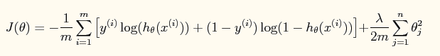
此时加入了规则项后的系统的损失函数为：

Newton’s method

Recall that the Newton's Method update rule is

$egin{displaymath} heta^{(t+1)}= heta^{(t)}-H^{-1} abla_{ heta}J onumber end{displaymath}$

$egin{displaymath} abla_{ heta}J = left[egin{array}{c} frac{1}{m}sum_{i... ...ight)x_{n}^{(i)}+frac{lambda}{m} heta_{n}end{array} ight] end{displaymath}$

$egin{displaymath} H & = & frac{1}{m}left[sum_{i=1}^{m}h_{ heta}(x^{(i)})l... ...}{cccc} 0\ & 1\ & & ddots\ & & & 1end{array} ight] end{displaymath}$

1. $x^{(i)}$ is your feature vector, which is a 28x1 vector in this exercise.

2. $abla_{ heta}J$ is a 28x1 vector.

3. $x^{(i)}(x^{(i)})^T$ and are 28x28 matrices.

4. $y^{(i)}$ and $h_ heta(x^{(i)})$ are scalars.

5. The matrix following $frac{lambda}{m}$ in the Hessian formula is a 28x28 diagonal matrix with a zero in the upper left and ones on every other diagonal entry.

After convergence, use your values of theta to find the decision boundary in the classification problem. The decision boundary is defined as the line where

$egin{displaymath} P(y=1vert x; heta) = 0.5 ;;;;; Longrightarrow ;;;;; heta^T x = 0 onumber end{displaymath}$

Code

%载入数据
clc,clear,close all;
x = load('ex5Logx.dat');
y = load('ex5Logy.dat');

%画出数据的分布图
plot(x(find(y),1),x(find(y),2),'o','MarkerFaceColor','b')
hold on;
plot(x(find(y==0),1),x(find(y==0),2),'r+')
legend('y=1','y=0')

% Add polynomial features to x by 
% calling the feature mapping function
% provided in separate m-file
x = map_feature(x(:,1), x(:,2));  %投影到高维特征空间

[m, n] = size(x);

% Initialize fitting parameters
theta = zeros(n, 1);

% Define the sigmoid function
g = inline('1.0 ./ (1.0 + exp(-z))'); 

% setup for Newton's method
MAX_ITR = 15;
J = zeros(MAX_ITR, 1);

% Lambda is the regularization parameter
lambda = 1;%lambda=0,1,10，修改这个地方，运行3次可以得到3种结果。

% Newton's Method
for i = 1:MAX_ITR
    % Calculate the hypothesis function
    z = x * theta;
    h = g(z);
    
    % Calculate J (for testing convergence) -- 损失函数
    J(i) =(1/m)*sum(-y.*log(h) - (1-y).*log(1-h))+ ...
    (lambda/(2*m))*norm(theta([2:end]))^2;
    
    % Calculate gradient and hessian.
    G = (lambda/m).*theta; G(1) = 0; % extra term for gradient
    L = (lambda/m).*eye(n); L(1) = 0;% extra term for Hessian
    grad = ((1/m).*x' * (h-y)) + G;
    H = ((1/m).*x' * diag(h) * diag(1-h) * x) + L;
    
    % Here is the actual update
    theta = theta - Hgrad;
  
end

% Plot the results 
% We will evaluate theta*x over a 
% grid of features and plot the contour 
% where theta*x equals zero

% Here is the grid range
u = linspace(-1, 1.5, 200);
v = linspace(-1, 1.5, 200);

z = zeros(length(u), length(v));
% Evaluate z = theta*x over the grid
for i = 1:length(u)
    for j = 1:length(v)
        z(i,j) = map_feature(u(i), v(j))*theta;%这里绘制的并不是损失函数与迭代次数之间的曲线，而是线性变换后的值
    end
end
z = z'; % important to transpose z before calling contour

% Plot z = 0
% Notice you need to specify the range [0, 0]
contour(u, v, z, [0, 0], 'LineWidth', 2)%在z上画出为0值时的界面，因为为0时刚好概率为0.5，符合要求
legend('y = 1', 'y = 0', 'Decision boundary')
title(sprintf('\lambda = %g', lambda), 'FontSize', 14)


hold off

% Uncomment to plot J
% figure
% plot(0:MAX_ITR-1, J, 'o--', 'MarkerFaceColor', 'r', 'MarkerSize', 8)
% xlabel('Iteration'); ylabel('J')

Result