【tensorflow】Tensorflow入门教程

原来链接 -> link

声明：

1. 参考自Python TensorFlow Tutorial – Build a Neural Network，本文简化了文字部分
2. 文中有很多到官方文档的链接，毕竟有些官方文档是中文的，而且写的很好。

Tensorflow入门

资源：付费tensorflow教程

Tensorflow graphs

Tensorflow是基于graph的并行计算模型。关于graph的理解可以参考官方文档。举个例子，计算a=(b+c)∗(c+2)a=(b + c) * (c + 2)a=(b+c)∗(c+2)，我们可以将算式拆分成一下：

d = b + c
e = c + 2
a = d * e

转换成graph后的形式为：


> 讲一个简单的算式搞成这样确实大材小用，但是我们可以通过这个例子发现：$d = b + c$和$e = c + 2$是不相关的，也就是可以**并行计算**。对于更复杂的CNN和RNN，graph的并行计算的能力将得到更好的展现。

实际中，基于Tensorflow构建的三层（单隐层）神经网络如下图所示：

 **Tensorflow data flow graph**

上图中，圆形或方形的节点被称为node，在node中流动的数据流被称为张量(tensor)。更多关于tensor的描述见官方文档。

0阶张量 == 标量
1阶张量 == 向量（一维数组）
2阶张量 == 二维数组
…
n阶张量 == n维数组

tensor与node之间的关系：
  如果输入tensor的维度是5000×645000 imes 645000×64，表示有5000个训练样本，每个样本有64个特征，则输入层必须有64个node来接受这些特征。

上图表示的三层网络包括：输入层(图中的input)、隐藏层(这里取名为ReLU layer表示它的激活函数是ReLU）、输出层(图中的Logit Layer)。

可以看到，每一层中都有相关tensor流入Gradient节点计算梯度，然后这些梯度tensor进入SGD Trainer节点进行网络优化（也就是update网络参数）。

Tensorflow正是通过graph表示神经网络，实现网络的并行计算，提高效率。下面我们将通过一个简单的例子来介绍TensorFlow的基础语法。

A Simple TensorFlow example

用Tensorflow计算a=(b+c)∗(c+2)a = (b + c) * (c + 2)a=(b+c)∗(c+2)， 1. 定义数据：

import tensorflow as tf

# 首先，创建一个TensorFlow常量=>2
const = tf.constant(2.0, name='const')

# 创建TensorFlow变量b和c
b = tf.Variable(2.0, name='b')
c = tf.Variable(1.0, dtype=tf.float32, name='c')

如上，TensorFlow中，使用tf.constant()定义常量，使用tf.Variable()定义变量。Tensorflow可以自动进行数据类型检测，比如：赋值2.0就默认为tf.float32，但最好还是显式地定义。更多关于TensorFlow数据类型的介绍查看官方文档。
2. 定义运算(也称TensorFlow operation)：

# 创建operation
d = tf.add(b, c, name='d')
e = tf.add(c, const, name='e')
a = tf.multiply(d, e, name='a')

发现了没，在TensorFlow中，+−×÷+- imes div+−×÷都有其特殊的函数表示。实际上，TensorFlow定义了足够多的函数来表示所有的数学运算，当然也对部分数学运算进行了运算符重载，但保险起见，我还是建议你使用函数代替运算符。

**！！TensorFlow中所有的变量必须经过初始化才能使用，**初始化方式分两步：

1. 定义初始化operation
2. 运行初始化operation

# 1. 定义init operation
init_op = tf.global_variables_initializer()

以上已经完成TensorFlow graph的搭建，下一步即计算并输出。

运行graph需要先调用tf.Session()函数创建一个会话(session)。session就是我们与graph交互的handle。更多关于session的介绍见官方文档。

# session
with tf.Session() as sess:
	# 2. 运行init operation
	sess.run(init_op)
	# 计算
	a_out = sess.run(a)
	print("Variable a is {}".format(a_out))

值得一提的是，TensorFlow有一个极好的可视化工具TensorBoard，详见官方文档。将上面例子的graph可视化之后的结果为：


The TensorFlow placeholder

对上面例子的改进：使变量b可以接收任意值。TensorFlow中接收值的方式为占位符(placeholder)，通过tf.placeholder()创建。

# 创建placeholder
b = tf.placeholder(tf.float32, [None, 1], name='b')

•  

第二个参数值为[None, 1]，其中None表示不确定，即不确定第一个维度的大小，第一维可以是任意大小。特别对应tensor数量(或者样本数量)，输入的tensor数目可以是32、64…

现在，如果得到计算结果，需要在运行过程中feed占位符b的值，具体为将a_out = sess.run(a)改为：

np.newaxis: https://www.jianshu.com/p/78e1e281f698

a_out = sess.run(a, feed_dict={b: np.arange(0, 10)[:, np.newaxis]})

输出：

Variable a is [[  3.]
 [  6.]
 [  9.]
 [ 12.]
 [ 15.]
 [ 18.]
 [ 21.]
 [ 24.]
 [ 27.]
 [ 30.]]

A Neural Network Example

神经网络的例子，数据集为MNIST数据集。
1. 加载数据：

from tensorflow.examples.tutorials.mnist import input_data
mnist = input_data.read_data_sets("MNIST_data/", one_hot=True)

•  

one_hot=True表示对label进行one-hot编码，比如标签4可以表示为[0, 0, 0, 0, 1, 0, 0, 0, 0, 0]。这是神经网络输出层要求的格式。

Setting things up

2. 定义超参数和placeholder

# 超参数
learning_rate = 0.5
epochs = 10
batch_size = 100

# placeholder
# 输入图片为28 x 28 像素 = 784
x = tf.placeholder(tf.float32, [None, 784])
# 输出为0-9的one-hot编码
y = tf.placeholder(tf.float32, [None, 10])

再次强调，[None, 784]中的None表示任意值，特别对应tensor数目。

3. 定义参数w和b

# hidden layer => w, b
W1 = tf.Variable(tf.random_normal([784, 300], stddev=0.03), name='W1')
b1 = tf.Variable(tf.random_normal([300]), name='b1')
# output layer => w, b
W2 = tf.Variable(tf.random_normal([300, 10], stddev=0.03), name='W2')
b2 = tf.Variable(tf.random_normal([10]), name='b2')

在这里，要了解全连接层的两个参数w和b都是需要随机初始化的，tf.random_normal()生成正态分布的随机数。

4. 构造隐层网络

# 计算输出
y_ = tf.nn.softmax(tf.add(tf.matmul(hidden_out, W2), b2))

上面代码对应于公式：

5. 构造输出（预测值）

<span style="color:#000000"><code># 计算输出
y_ = tf.nn.softmax(tf.add(tf.matmul(hidden_out, W2), b2))
</code></span>

对于单标签多分类任务，输出层的激活函数都是tf.nn.softmax()。更多关于softmax的知识见维基百科。

6. BP部分—定义loss
损失为交叉熵，公式为

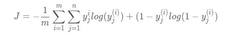
公式分为两步：

1. 对n个标签计算交叉熵
2. 对m个样本取平均

•  

7. BP部分—定义优化算法

# 创建优化器，确定优化目标
optimizer = tf.train.GradientDescentOptimizer(learning_rate=learning_rate).minimizer(cross_entropy)

TensorFlow中更多优化算法详见官方文档。

8. 定义初始化operation和准确率node

# init operator
init_op = tf.global_variables_initializer()

# 创建准确率节点
correct_prediction = tf.equal(tf.argmax(y, 1), tf.argmax(y_, 1))
accuracy = tf.reduce_mean(tf.cast(correct_prediction, tf.float32))

correct_predicion会返回一个m×1m imes 1m×1的tensor，tensor的值为True/False表示是否正确预测。

Setting up the training

9. 开始训练

# 创建session
with tf.Session() as sess:
	# 变量初始化
	sess.run(init_op)
	total_batch = int(len(mnist.train.labels) / batch_size)
	for epoch in range(epochs):
		avg_cost = 0
		for i in range(total_batch):
			batch_x, batch_y = mnist.train.next_batch(batch_size=batch_size)
			_, c = sess.run([optimizer, cross_entropy], feed_dict={x: batch_x, y: batch_y})
			avg_cost += c / total_batch
		print("Epoch:", (epoch + 1), "cost = ", "{:.3f}".format(avg_cost))
	print(sess.run(accuracy, feed_dict={x: mnist.test.images, y: mnist.test.labels}))

输出：

<span style="color:#000000"><code>Epoch: 1 cost = 0.586
Epoch: 2 cost = 0.213
Epoch: 3 cost = 0.150
Epoch: 4 cost = 0.113
Epoch: 5 cost = 0.094
Epoch: 6 cost = 0.073
Epoch: 7 cost = 0.058
Epoch: 8 cost = 0.045
Epoch: 9 cost = 0.036
Epoch: 10 cost = 0.027

Training complete!
0.9787
</code></span>

通过TensorBoard可视化训练过程：