协同过滤与奇异值分解
1. Introduction
A recommender system refers to a system that is capable of predicting the future preference of a set of items for a user, and recommend the top items. One key reason why we need a recommender system in modern society is that people have too much options to use from due to the prevalence of Internet. In the past, people used to shop in a physical store, in which the items available are limited. For instance, the number of movies that can be placed in a Blockbuster store depends on the size of that store. By contrast, nowadays, the Internet allows people to access abundant resources online. Netflix, for example, has an enormous collection of movies. Although the amount of available information increased, a new problem arose as people had a hard time selecting the items they actually want to see. This is where the recommender system comes in. This article will give you a brief introduction to two typical ways for building a recommender system, Collaborative Filtering and Singular Value Decomposition.

2. Traditional Approach
Traditionally, there are two methods to construct a recommender system :
- Content-based recommendation
- Collaborative Filtering
The first one analyzes the nature of each item. For instance, recommending poets to a user by performing Natural Language Processing on the content of each poet. Collaborative Filtering, on the other hand, does not require any information about the items or the users themselves. It recommends items based on users' past behavior. I will elaborate more on Collaborative Filtering in the following paragraphs.
3. Collaborative Filtering
As mentioned above, Collaborative Filtering (CF) is a mean of recommendation based on users' past behavior. There are two categories of CF:
- User-based: measure the similarity between target users and other users
- Item-based: measure the similarity between the items that target users rates/ interacts with and other items
The key idea behind CF is that similar users share the same interest and that similar items are liked by a user.
Assume there are m users and n items, we use a matrix with size m*n to denote the past behavior of users. Each cell in the matrix represents the associated opinion that a user holds. For instance, M_{i, j} denotes how user i likes item j. Such matrix is called utility matrix. CF is like filling the blank (cell) in the utility matrix that a user has not seen/rated before based on the similarity between users or items. There are two types of opinions, explicit opinion and implicit opinion. The former one directly shows how a user rates that item (think of it as rating an app or a movie), while the latter one only serves as a proxy which provides us heuristics about how an user likes an item (e.g. number of likes, clicks, visits). Explicit opinion is more straight-forward than the implicit one as we do not need to guess what does that number implies. For instance, there can be a song that user likes very much, but he listens to it only once because he was busy while he was listening to it. Without explicit opinion, we cannot be sure whether the user dislikes that item or not. However, most of the feedback that we collect from users are implicit. Thus, handling implicit feedback properly is very important, but that is out of the scope of this blog post. I'll move on and discuss how CF works.
User-based Collaborative Filtering
We know that we need to compute the similarity between users in user-based CF. But how do we measure the similarity? There are two options, Pearson Correlation or cosine similarity. Let u_{i, k} denotes the similarity between user i and user k and v_{i, j} denotes the rating that user i gives to item j with v_{i, j} = ? if the user has not rated that item. These two methods can be expressed as the followings:
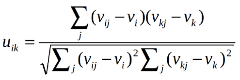
Both measures are commonly used. The difference is that Pearson Correlation is invariant to adding a constant to all elements.

Now, we can predict the users' opinion on the unrated items with the below equation:

Let me illustrate it with a concrete example. In the following matrixes, each row represents a user, while the columns correspond to different movies except the last one which records the similarity between that user and the target user. Each cell represents the rating that the user gives to that movie. Assume user E is the target.
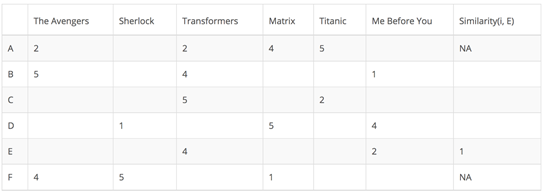
Since user A and F do not share any movie ratings in common with user E, their similarities with user E are not defined in Pearson Correlation. Therefore, we only need to consider user B, C, and D. Based on Pearson Correlation, we can compute the following similarity.
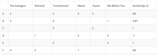
From the above table you can see that user D is very different from user E as the Pearson Correlation between them is negative. He rated Me Before You higher than his rating average, while user E did the opposite. Now, we can start to fill in the blank for the movies that user E has not rated based on other users.

Although computing user-based CF is very simple, it suffers from several problems. One main issue is that users' preference can change over time. It indicates that precomputing the matrix based on their neighboring users may lead to bad performance. To tackle this problem, we can apply item-based CF.
Item-based Collaborative Filtering
Instead of measuring the similarity between users, the item-based CF recommends items based on their similarity with the items that the target user rated. Likewise, the similarity can be computed with Pearson Correlation or Cosine Similarity. The major difference is that, with item-based collaborative filtering, we fill in the blank vertically, as oppose to the horizontal manner that user-based CF does. The following table shows how to do so for the movie Me Before You.
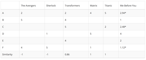
It successfully avoids the problem posed by dynamic user preference as item-based CF is more static. However, several problems remain for this method. First, the main issue is scalability. The computation grows with both the customer and the product. The worst case complexity is O(mn) with m users and n items. In addition, sparsity is another concern. Take a look at the above table again. Although there is only one user that rated both Matrix and Titanic rated, the similarity between them is 1. In extreme cases, we can have millions of users and the similarity between two fairly different movies could be very high simply because they have similar rank for the only user who ranked them both.
4. Singular Value Decomposition
One way to handle the scalability and sparsity issue created by CF is to leverage a latent factor model to capture the similarity between users and items. Essentially, we want to turn the recommendation problem into an optimization problem. We can view it as how good we are in predicting the rating for items given a user. One common metric is Root Mean Square Error (RMSE). The lower the RMSE, the better the performance. Since we do not know the rating for the unseen items, we will temporarily ignore them. Namely, we are only minimizing RMSE on the known entries in the utility matrix. To achieve minimal RMSE, Singular Value Decomposition (SVD) is adopted as shown in the below formula.
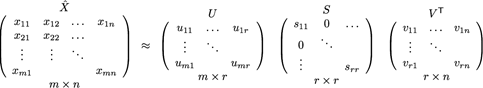
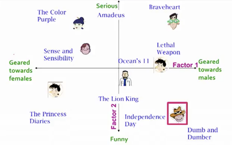
X denotes the utility matrix, and U is a left singular matrix, representing the relationship between users and latent factors. S is a diagonal matrix describing the strength of each latent factor, while V transpose is a right singular matrix, indicating the similarity between items and latent factors. Now, you might wonder what do I mean by latent factor here? It is a broad idea which describes a property or concept that a user or an item have. For instance, for music, latent factor can refer to the genre that the music belongs to. SVD decreases the dimension of the utility matrix by extracting its latent factors. Essentially, we map each user and each item into a latent space with dimension r. Therefore, it helps us better understand the relationship between users and items as they become directly comparable. The below figure illustrates this idea.
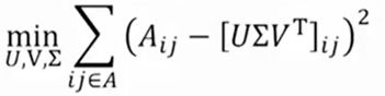
SVD has a great property that it has the minimal reconstruction Sum of Square Error (SSE); therefore, it is also commonly used in dimensionality reduction. The below formula replace X with A, and S with Σ.
But how does this has to do with RMSE that I mentioned at the beginning of this section? It turns out that RMSE and SSE are monotonically related. This means that the lower the SSE, the lower the RMSE. With the convenient property of SVD that it minimizes SSE, we know that it also minimizes RMSE. Thus, SVD is a great tool for this optimization problem. To predict the unseen item for a user, we simply multiply U, Σ, and T.
Python Scipy has a nice implementation of SVD for sparse matrix.
>>> from
scipy.sparse
import csc_matrix
>>> from
scipy.sparse.linalg
import svds
>>> A = csc_matrix([[1, 0, 0], [5, 0, 2], [0, -1, 0], [0, 0, 3]], dtype=float)
>>> u, s, vt = svds(A, k=2) # k is the number of factors
>>> s
array([ 2.75193379, 5.6059665 ])
SVD handles the problem of scalability and sparsity posed by CF successfully. However, SVD is not without flaw. The main drawback of SVD is that there is no to little explanation to the reason that we recommend an item to an user. This can be a huge problem if users are eager to know why a specific item is recommended to them. I will talk more on that in the next blog post.
5. Conclusion
I have discussed two typical methods for building a recommender system, Collaborative Filtering and Singular Value Decomposition. In the next blog post, I will continue to talk about some more advanced algorithms for building a recommender system.
1。介绍
推荐系统指的是能够预测用户对一组项目未来偏好的系统,并推荐顶级项目。在现代社会中,我们需要一个推荐系统的一个关键原因是,由于因特网的普及,人们有太多的选择可以使用。过去,人们过去常在实体店购物,因为那里的商品有限。例如,可以放在大片商店里的电影数量取决于那家商店的规模。相比之下,如今,互联网允许人们在网上获取丰富的资源。例如,Netflix有大量的电影收藏。虽然可用信息的数量增加了,但新的问题出现了,因为人们很难选择他们真正想要看到的东西。推荐系统就在这里。本文将简要介绍两种典型的构建推荐系统的方法:协同过滤和奇异值分解。
________________________________________
2。传统的方法
传统上,推荐方法有两种构造方法:
•基于内容的推荐
•协同过滤
第一个是分析每个项目的性质。例如,通过对每个诗人的内容进行自然语言处理,向用户推荐诗人。另一方面,协作过滤不需要关于项目或用户本身的任何信息。它根据用户过去的行为推荐项目。在下面的段落中,我将详细讨论协作过滤。
三.协同过滤
如上所述,协同过滤(CF)是一种基于用户过去行为的推荐方法。有两类CF:
•基于用户:测量目标用户和其他用户之间的相似性
•基于项目:测量目标用户与其他项目之间的相似性
CF背后的关键思想是相似的用户共享相同的兴趣,用户喜欢类似的项目。
假设有m个用户和n个项,我们使用一个大小为m×n的矩阵来表示用户过去的行为。矩阵中的每个单元格表示用户持有的相关意见。例如,m_ {i,j}表示用户我喜欢项J.这样的矩阵称为效用矩阵。CF类似于在用户或项目之间基于用户或用户之间的相似性在用户面前没有看到/评估的效用矩阵中的空白(单元格)。有两种意见,一种是明确的意见,一种是隐含的意见。前者直接显示用户如何评价该项(把它看作是一个应用程序或一个电影),而后者只是作为一个代理,它为我们提供了一个关于用户如何喜欢一个项目的启发式(例如,喜欢,点击,访问次数)。明确的观点比隐含的观点更直接,因为我们不需要猜测这个数字意味着什么。例如,可以有一首歌,用户非常喜欢,但他只听一次,因为他在听的时候很忙。没有明确的意见,我们不能确定用户是否讨厌这个项目。然而,我们从用户那里收集的大部分反馈是隐含的。因此,正确地处理隐含反馈是非常重要的,但这超出了这个博客文章的范围。我将继续讨论CF是如何工作的。
基于用户的协同过滤
我们知道,我们需要计算用户之间的相似性,以用户为基础的CF,但我们如何衡量的相似性?有两种选择,皮尔森相关性或余弦相似性。让我u_ { },K表示用户我和用户K和v_ {我之间的相似性,j}表示评级用户我给J项与v_ {i,j} =?如果用户没有对该项目进行评级。这两种方法可以表示如下:
这两种措施都是常用的。不同的是,皮尔森相关性是不变的,为所有元素添加一个常量。
现在,我们可以预测用户对未评分项目的意见,下面的方程:
让我用一个具体的例子来说明它。在下面的矩阵中,每一行表示一个用户,而列对应于不同的电影,除了最后一个记录该用户与目标用户之间的相似性的电影。每个单元格表示用户给该电影的评级。假定用户e是目标。
由于用户A和F不与用户E共享任何电影等级,它们与用户e的相似性没有在皮尔森相关中定义。因此,我们只需要考虑基于皮尔森相关的用户B、C和D,就能计算出以下相似性。
从上面的表可以看出,用户d与用户E非常不同,因为它们之间的皮尔森相关性是负的。他比你的评级平均高出我,而用户E则相反。现在,我们可以开始填补空白的电影用户E没有根据其他用户的评级。
虽然计算基于用户的CF很简单,但它有几个问题。一个主要问题是用户的偏好随时间而变化。结果表明,预计算基于相邻用户的矩阵会导致不好的表现。为了解决这个问题,我们可以应用基于项的CF。
基于项目的协同过滤
不是基于用户之间的相似性度量,基于项目的CF推荐基于与目标用户评分的项目相似性的项目。同样,相似度可以用皮尔森相关或余弦相似性来计算。主要区别在于,基于项目的协作过滤,我们垂直地填充空白,与基于用户的CF的横向方式相反。下表显示了如何在我之前为我拍摄电影。
它成功地避免了动态用户偏好所带来的问题,因为基于项的CF更静态。然而,这种方法仍然存在一些问题。首先,主要问题是可伸缩性。计算随着客户和产品的增长而增长。最坏情况下的复杂度是O(MN)与m用户和n项。此外,稀疏性是另一个问题。再看一下上面的表格。虽然只有一个用户额定矩阵和泰坦尼克号,他们之间的相似性是1。在极端情况下,我们可以拥有数以百万计的用户,而两部截然不同的电影之间的相似性可能非常高,因为它们对于排名第二的唯一用户具有相似的排名。
4。奇异值分解
处理CF创建的可伸缩性和稀疏性问题的一种方法是利用潜在因素模型来捕获用户和项目之间的相似性。本质上,我们希望把推荐问题转化为最优化问题。我们可以把它看作是我们在预测用户给定项目的评级方面有多好。一个常见的度量是均方根误差(RMSE)。均方根误差较低,性能就越好。由于我们不知道无形物品的评级,我们将暂时忽略它们。即,我们在效用矩阵最小RMSE在已知的条目。实现最小RMSE、奇异值分解(SVD)采用以下公式所示。
x表示效用矩阵,u是一个左奇异矩阵,表示用户与潜在因素之间的关系。s是描述每个潜在因子强度的对角矩阵,而v转置是一个右奇异矩阵,表示项和潜因子之间的相似性。现在,你可能想知道这里的潜在因素是什么意思吗?这是一个宽泛的概念,它描述用户或项目拥有的属性或概念。例如,对于音乐来说,潜在因素可以指音乐属于的类型。奇异值分解通过提取潜在因素来减少效用矩阵的维数。本质上,我们将每个用户和每个项目映射成一个带有维度r的潜在空间,因此,它可以帮助我们更好地理解用户和项目之间的关系,因为它们可以直接比较。下图说明了这个想法。
奇异值分解有一个大的性质,它具有最小的平方和重构(SSE),因此,它也常用于降维。下面的公式代替x,和SΣ。
但这样会有误差,我提到在本节开始的吗?原来,RMSE和SSE是单调相关。这意味着,上交所降低,较低的均方根误差。用奇异值分解的方便性,它最大限度地减少SSE,我们知道它也最小化RMSE。因此,SVD是这个优化问题的一个很好的工具。预测看不见的项目的用户,我们只要把U,Σ,和T.
Python SciPy具有稀疏矩阵的奇异值分解的一个很好的实现。
> > >从scipy.sparse进口csc_matrix
> > >从scipy.sparse.linalg进口SVDs
> > > = csc_matrix([ [ 1, 0, 0 ]、[ 5, 0, 2 ]、[ 0,1, 0 ],[ 0, 0, 3 ] ],D =浮动)
> > > U,S,VT = SVDs(A,k = 2)# K因子的数量
> >
数组([ 2.75193379,5.6059665 ])
奇异值分解处理CF所带来的可伸缩性和稀疏性问题。然而,SVD并非没有缺陷。SVD的主要缺点是对我们向用户推荐一个项目的原因没有什么解释。如果用户急于知道为什么推荐一个特定的项目,这将是一个巨大的问题。我会在下一篇博文中详细讨论这个问题。
5。结论
讨论了建立推荐系统的两种典型方法:协同过滤和奇异值分解。在下一篇博客文章中,我将继续讨论一些更高级的构建推荐系统的算法。