必做:
[*] warmUpExercise.m - Simple example function in Octave/MATLAB
[*] plotData.m - Function to display the dataset
[*] computeCost.m - Function to compute the cost of linear regression
[*] gradientDescent.m - Function to run gradient descent
1.warmUpExercise.m
A = eye(5);
2.plotData.m
plot(x, y, 'rx', 'MarkerSize', 10); % Plot the data
ylabel('Profit in $10,000s'); % Set the y-axis label
xlabel('Population of City in 10,000s'); % Set the x-axis label
3.computeCost.m
function J = computeCost(X, y, theta)
%COMPUTECOST Compute cost for linear regression
%   J = COMPUTECOST(X, y, theta) computes the cost of using theta as the
%   parameter for linear regression to fit the data points in X and y

% Initialize some useful values
m = length(y); % number of training examples

% You need to return the following variables correctly
J = 0;

% ====================== YOUR CODE HERE ======================
% Instructions: Compute the cost of a particular choice of theta
%               You should set J to the cost.

H = X*theta-y;
J = (1/(2*m))*sum(H.*H);

% =========================================================================

end
公式: 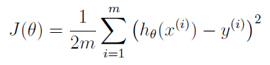
注意matlab中 .* 的用法。
4.gradientDescent.m
function [theta, J_history] = gradientDescent(X, y, theta, alpha, num_iters)
%GRADIENTDESCENT Performs gradient descent to learn theta
%   theta = GRADIENTDESCENT(X, y, theta, alpha, num_iters) updates theta by
%   taking num_iters gradient steps with learning rate alpha

% Initialize some useful values
m = length(y); % number of training examples
J_history = zeros(num_iters, 1);

for iter = 1:num_iters

    % ====================== YOUR CODE HERE ======================
    % Instructions: Perform a single gradient step on the parameter vector
    %               theta.
    %
    % Hint: While debugging, it can be useful to print out the values
    %       of the cost function (computeCost) and gradient here.

     H = X*theta-y;
    theta(1)=theta(1)-alpha*(1/m)*sum(H.*X(:,1));
    theta(2)=theta(2)-alpha*(1/m)*sum(H.*X(:,2));

    % ============================================================

    % Save the cost J in every iteration
    J_history(iter) = computeCost(X, y, theta);

end

end
单变量梯度下降
对函数J(θ)求偏导
![]()
即 H.*X(:,1)
θi向着梯度最小的方向减少,alpha为步长。
![]()
theta(i)=theta(i)-alpha*(1/m)*sum(H.*X(:,i));