Coursera Machine Learning-Andrew Ng 学习笔记
所有图片来自视频截图
部分表述也是原视频表述
what is machine learning?
“The field of study that gives computers the ability to learn without being explicitly programmed.” —-Arthur Samuel
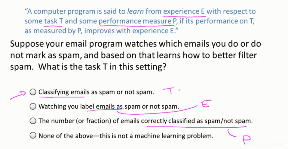
“A computer program is said to learn from experience E, with respect to some task T, and some performance measure P, if its performance on T as measured by P improves with experience E. ” —–Tom Mitchell
Two class machine learning method
In general, any machine learning problem can be assigned to one of two broad classifications:
Supervised learning and Unsupervised learning.
Supervised learning
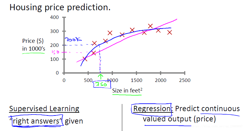
example 1: regression problem
Given data about the size of houses on the real estate market, try to predict their price. Price as a function of size is a continuous output, so this is a regression problem.
example 2: classification problem
Given a patient with a tumor, we have to predict whether the tumor is malignant or benign.
The sample has been labeled as discrete valued(0 OR 1).
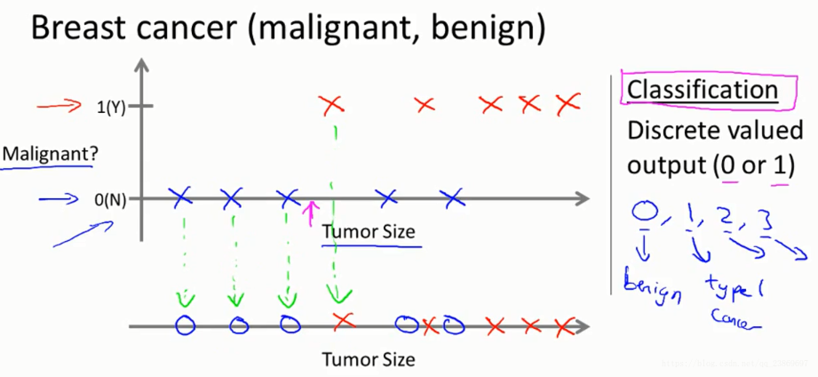
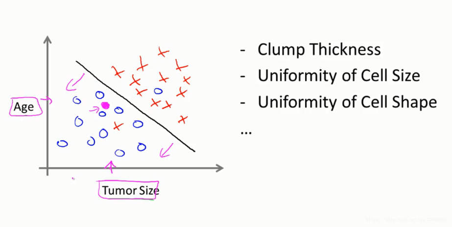
Classify the breast cancer with two or more features.
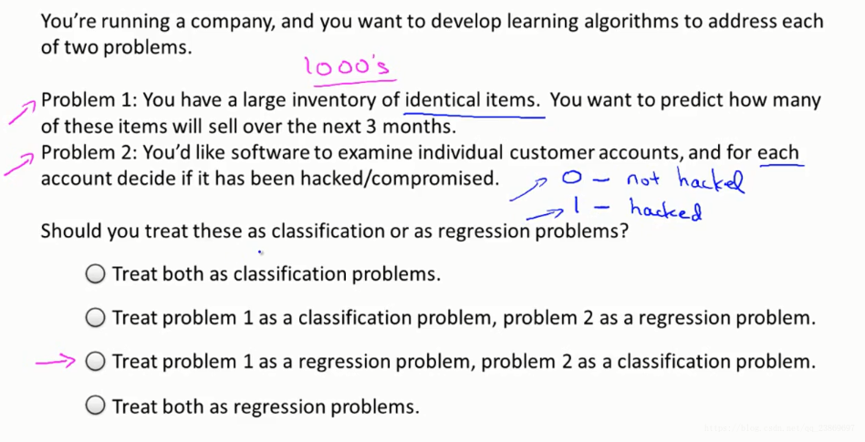
The different between regression and classification
In regression problem, we are going to map input variables to some continuous function, but in classification problem, to discrete categories.
Unsupervised learning
Allow you to derive structure from data where we don’t know the result.
example: clustering
Group the genes
example: non clustering
identifying individual voices and music from a mesh of sounds at a cocktail party
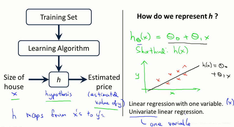
model representation
本课程使用的标注
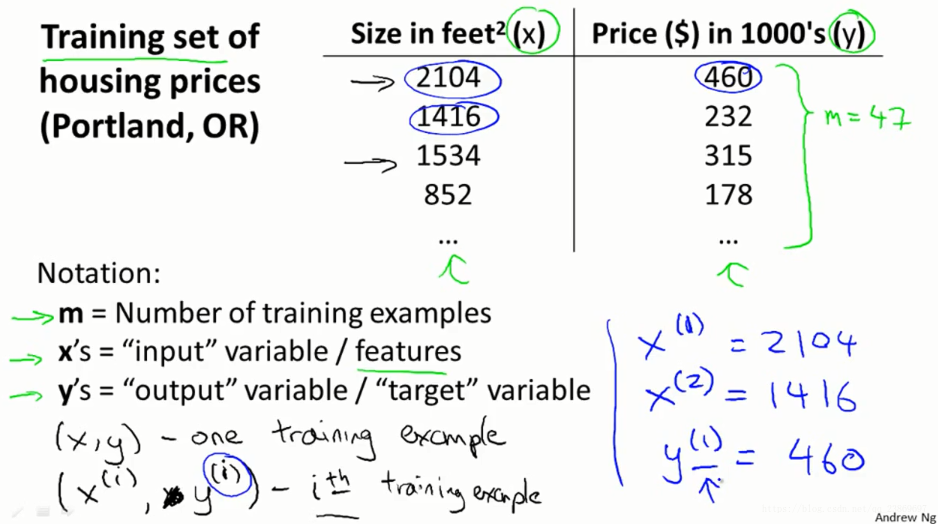
模型
给定一个训练集,我们的目标是是去学习一个函数h:x->y.
Cost function 1
在上面房价和面积的问题中,我们想弄清楚如何把最可能的直线与我们的数据拟合。在这个线性模型中,有两个参数θ0和θ1 ,如何选择这两个参数值θ0和θ1就是我们这个问题的关键,下面不同的取值有不同的结果。
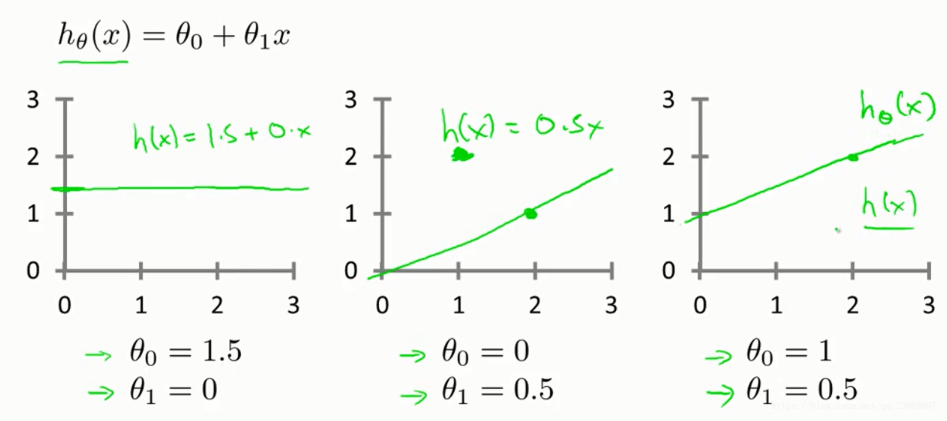
如何选择这两个参数?
简单的想法就是: 选择一条直线使所有的点距离这条直线最近。
用什么来衡量这个最近?
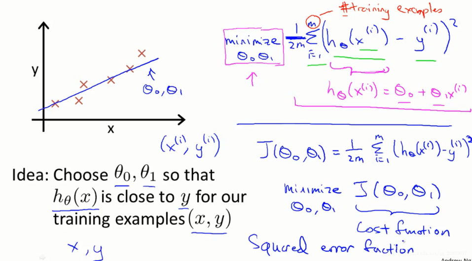
每一个样本的预测值减去样本的真实值的平方, 再把所有差的平方相加得到总和,除以样本个数m得到其均值。为便于后续的计算,我们常再乘以。这就是常用的均方差。
我们把这函数定义为代价函数,所以在这里,代价函数等同于平方误差函数。
我们的目标变成了求代价函数在参数取何值时取得最小值问题。
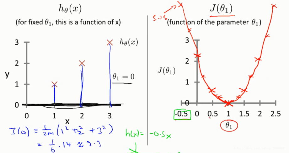
Cost function 2
我们先假设只有一个参数的情况:
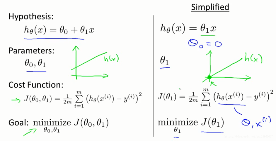
不同的取值有不同的, 所以能够画出的图像,如右图。
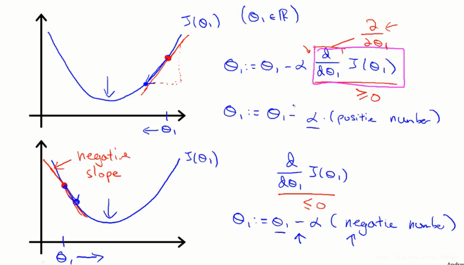
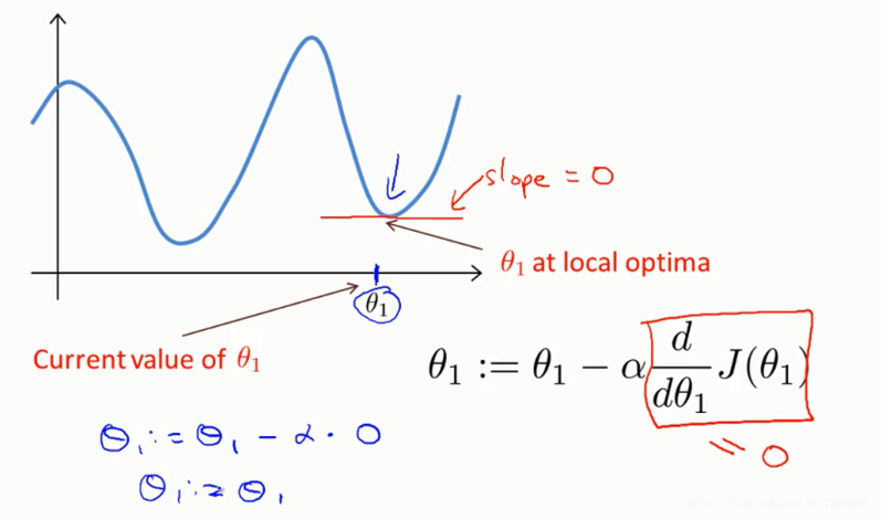
Gradient Descent 1
我们先从简单的两个参数开始介绍梯度下降算法。从图上理解梯度下降:
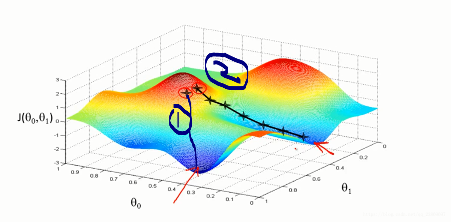
我们也能从图中看到,梯度下降的方向不一样,我们不一定达到全局的最小值,可能找到的局部最小值。
从算法理解梯度下降:
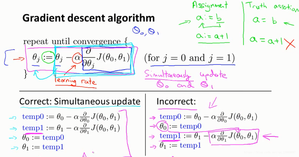
赋值符号使用 := 而不是=.
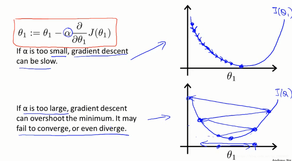
这里的α是一个数字,被称为学习速率。在梯度下降算法中 它控制我们下山时会迈出多大的步子。 因此如果 α值很大,那么相应的梯度下降过程中,我们会试图用大步子下山 。如果α值很小,那么我们会迈着很小的小碎步下山,关于如何设置 α的值等内容,在之后的课程中会讲。
梯度下降的过程就是不断更新, 的过程,直到他们不再改变。
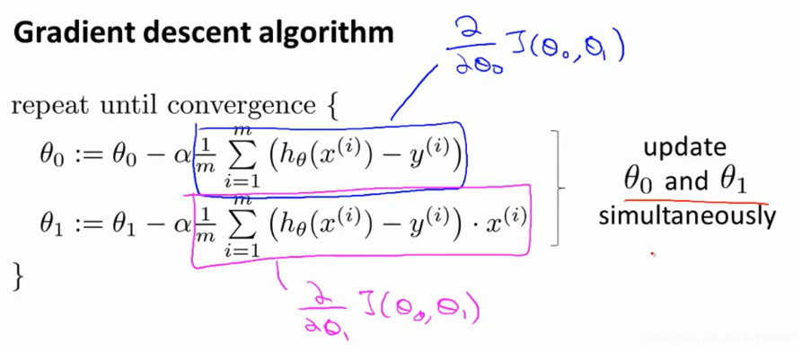
算法中, 必须同时更新。
Gradient Descent 2
梯度下降算法详解
假设我们只有一个参数:
考虑学习率带来的收敛缓慢和overshoot问题
为什么会找到局部极小值?
即使是固定学习率,当梯度在接近局部最小值或者全局最小值的时候或变得越来越小。
Gradient Descent For Linear Regression
使用梯度下降算法去解线性回归中的单价函数最小值问题。
将算法中的函数使用代替,也就是平方误差函数。
对平方误差中的参数分别求偏导再带入数据,不断迭代更新,直到不再改变就能找到最优值。
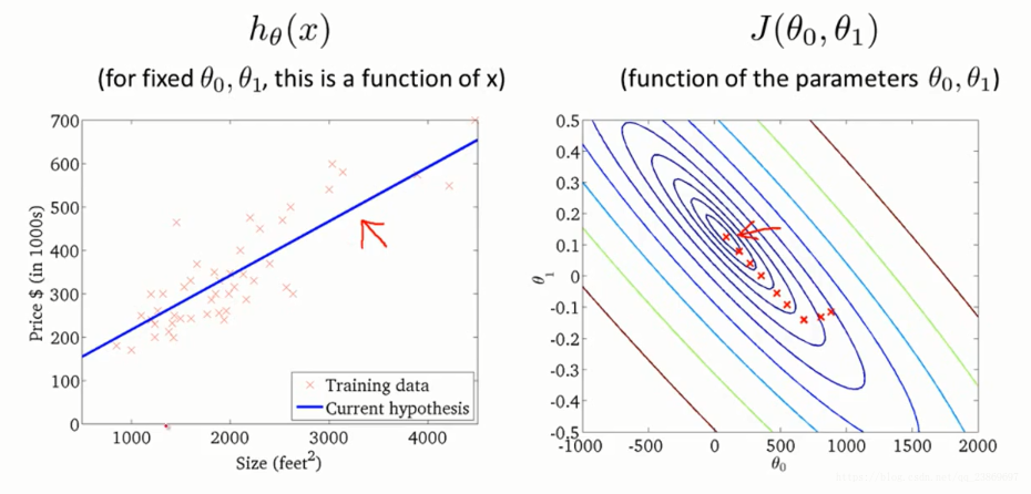
画出其三维图像:
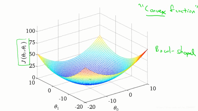
从轮廓图中看梯度的变化:
什么是“batch”?
“Batch” 梯度下降使用的是全部的数据,而深度学习里用的是一个子集,这个要注意区分。