问题1:扔下圆球的位置(feature特征变量)变化,最终掉落奖项(label结果标签)的变化
- feature ----输入
- f(x) ----模型,算法
- label ----输出
大量已知的数据,训练得出f(x)
- 一般的三步
- 收集数据feature,label
- 选择数据模型建立feature,label的关系--f(x)
- 根据选择的模型进行预测
- 人类建立模型:多次尝试增加经验提高预测到达公司的时间
- 机器学习:利用统计学,概率论,信息论的数学方法,利用已知的数据,创建一种模型,利用这种模型进行预测(高考与之类似)
- 机器学习经典模型:KNN模型(人以类聚,物以群分)
- 基本步骤
- 1.采集数据
- 2.计算实验数据与预测位置的距离
- 3.按照距离从小到大排序
- 4.选取最顶部的K条记录,得到最大概率的落点
- 5.预测预测位置的落点
- python实现
-
import numpy as np
import collections as c
# 1.采集数据
data = np.array([
	[154, 1],
	[126, 2],
	[70, 2],
	[196, 2],
	[161, 2],
	[371, 4],
])

# feature,label
feature = data[:, 0]
label = data[:, -1]

# 2.计算实验数据与预测点的距离
predictPoint = 200
distance = list(map(lambda x: abs(x - predictPoint), feature))

# 3.按照距离从小到大排序,排序下标
sortindex = np.argsort(distance)


# 4.选取最顶部的K条记录,得到最大概率的落点,假设K=3
sortedlabel = label[sortindex]
k = 3
# 预测结果[(结果,次数)]
# 5.预测预测位置的落点
predictlabel = c.Counter(sortedlabel[0:k]).most_common(1)[0][0]

print(predictlabel)
-
- 代码封装
-
import numpy as np
import collections as c


# 代码封装

def knn(k, predictPoint, feature, label):
	distance = list(map(lambda x: abs(x - predictPoint), feature))
	sortindex = np.argsort(distance)
	sortedlabel = label[sortindex]
	predictlabel = c.Counter(sortedlabel[0:k]).most_common(1)[0][0]
	return predictlabel


if __name__ == '__main__':
	data = np.array([
		[154, 1],
		[126, 2],
		[70, 2],
		[196, 2],
		[161, 2],
		[371, 4],
	])
	# feature,label
	feature = data[:, 0]
	label = data[:, -1]
	k = 3
	predictPoint = 200
	res = knn(k, predictPoint, feature, label)
	print(res)
-
- 实际数据验证
- 数据集https://pan.baidu.com/s/1rw5aFlVzZb6SBdY09Rckhg
-
import numpy as np import collections as c # 代码封装 def knn(k, predictPoint, feature, label): distance = list(map(lambda x: abs(x - predictPoint), feature)) sortindex = np.argsort(distance) sortedlabel = label[sortindex] predictlabel = c.Counter(sortedlabel[0:k]).most_common(1)[0][0] return predictlabel if __name__ == '__main__': data = np.loadtxt("数据集/data0.csv", delimiter=",") # feature,label feature = data[:, 0] label = data[:, -1] k = 3 predictPoint = 300 res = knn(k, predictPoint, feature, label) print(res) - 打散数据得到训练集和测试集
- import numpy as np
-
import collections as c # 代码封装 def knn(k, predictPoint, feature, label): distance = list(map(lambda x: abs(x - predictPoint), feature)) sortindex = np.argsort(distance) sortedlabel = label[sortindex] predictlabel = c.Counter(sortedlabel[0:k]).most_common(1)[0][0] return predictlabel if __name__ == '__main__': data = np.loadtxt("数据集/data0.csv", delimiter=",") # 打散数据 np.random.shuffle(data) # 训练90% traindata = data[100:-1] # 测试10% testdata = data[0:100] # 保存训练数据,测试数据 np.savetxt("data0-test.csv", testdata, delimiter=",", fmt="%d") np.savetxt("data0-train.csv", traindata, delimiter=",", fmt="%d") traindata = np.loadtxt("data0-train.csv", delimiter=",") # feature,label feature = traindata[:, 0] label = traindata[:, -1] max_accuracy = 0 max_k = [] # 预测点,来自测试数据的每一条记录 testdata = np.loadtxt("data0-test.csv", delimiter=",") for k in range(1,100): count = 0 for item in testdata: predict = knn(k, item[0], feature, label) real = item[1] if predict == real: count += 1 accuracy = count * 100.0 / len(testdata) if accuracy >= max_accuracy: max_accuracy = accuracy max_k.append(k) print("k = {},准确率:{}%".format(k,count*100.0/len(testdata))) print(set(max_k)) -
多维数据的距离的选取
-
欧式距离即可
-
- 预测不是很准确
- 1.模型的参数选择不够好,调参---调参工程师
- K选择太小,噪音干扰太明显
- K选择太大,其他类型的会涵盖
- K值的评价标准
- 训练集trainData---得到模型
- 测试集testData---验证模型
- 经验:K一般选取样本集开平方
- 2.影响因子不够多
- 增加数据的维度
- 球的颜色导致弹性不同
- 特殊数据的导入
-
import numpy as np

def colornum(str):
	dict = {"红":0.50,"黄":0.51,"蓝":0.52,"绿":0.53,"紫":0.54,"粉":0.55}
	return dict[str]


data = np.loadtxt('数据集/data1.csv',delimiter=",",converters={1:colornum},encoding="gbk")
print(data)
-
- 增加数据的维度
- 3.样本数据量不够
- 4.选择的模型不够好,选择其他机器学习的模型
- 1.模型的参数选择不够好,调参---调参工程师
- 基本步骤
- 线性回归
- 是一种总结规律,总结模型的解决方法。不需要全数据集
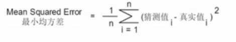
- 损失函数:评测算法的好坏
- 最小均方差
- 最小均方差越接近0越好
- 步骤
- 1.随机选取m和b
- 2.分别计算m和b的偏导数
- 3.如果m和b的偏导都很小,就成功
- 4.根据学习速率,计算出修改的值
- 5.b和m分别减去要修改的值
- python实import numpy as np
-
# data = np.array([ # [80, 200], # [95, 230], # [104, 245], # [112, 274], # [125, 259], # [135, 262], # ]) data = np.loadtxt('数据集/cars.csv', delimiter=",", skiprows=1, usecols=(4, 1)) m = 1 b = 1 xarray = data[:, 0] yreal = data[:, -1] learningrate = 0.00001 # 梯度下降 def grandentdecent(): # 求斜率 bslop = 0 for index, x in enumerate(xarray): bslop = bslop + m * x + b - yreal[index] bslop = bslop * 2 / len(xarray) # print("对b求导的斜率={}".format(bslop)) mslop = 0 for index, x in enumerate(xarray): mslop = mslop + (m * x + b - yreal[index]) * x mslop = mslop * 2 / len(xarray) # print("对m求导的斜率={}".format(mslop)) return (bslop, mslop) def train(): for i in range(1, 10000000): bslop, mslop = grandentdecent() global m m = m - mslop * learningrate global b b = b - bslop * learningrate if (abs(mslop) < 0.5 and abs(bslop) < 0.5): break print("m={},b={}".format(m, b)) if __name__ == '__main__': train() # 用训练集得到公式 # 用测试集验证正确率 -
import numpy as np

# 面积,房价
data = np.array([
	[80, 200],
	[95, 230],
	[104, 245],
	[112, 274],
	[125, 259],
	[135, 262],
])
# 1.feature,label,axis=1保留原始维度
feature = np.expand_dims(data[:, 0], axis=1)
# feature = data[:,0:1]
label = np.expand_dims(data[:, -1], axis=1)

# 2.weight
m = 1
b = 1

weight = np.array([
	[m],
	[b],
])
# 3.feature*weight,需要在feature后面补一列1---每一行代表mx+b
feature = np.append(feature, np.ones(shape=(6, 1)), axis=1)

print(feature)
# 4.feature*weight - label  得到差值difference
difference = np.dot(feature, weight) - label
# 5.feature^T*difference/n 先将feature转置在乘,得到对B和M的偏导bslop,mslop
bmslop = np.dot(feature.T, difference)
bmslop = bmslop*2/len(feature)
# 6.仅需使其数字接近0即可
-
图形变化
-
import matplotlib.pyplot as plt
import numpy as np
import math

points = np.array([
	[0, 0],
	[0, 5],
	[3, 5],
	[3, 4],
	[1, 4],
	[1, 3],
	[2, 3],
	[2, 2],
	[1, 2],
	[1, 0],
	[0, 0],
])
plt.plot(points[:, 0], points[:, 1])
for i in range(1,13):
	# # 1.平移
	# matrix = np.array([0.5*i, 0])
	# newpoints = points + matrix
	# 2.旋转
	# matrix = np.array([
	# 	[math.cos(math.pi/6),-math.sin(math.pi/6)],
	# 	[math.sin(math.pi/6),math.cos(math.pi/6)],
	# ])
	# points = np.dot(points,matrix)
	# 3.缩放
	matrix = np.array([
		[1.05,0],
		[0,1.05],
	])
	points = np.dot(points, matrix)
	plt.plot(points[:, 0], points[:, 1])
	plt.xlim(-10,10)
	plt.ylim(-10,10)
	plt.show()
-
-
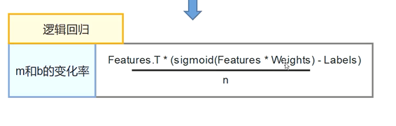
逻辑回归
-
将线性回归置于e的指数即可
-
e的求法
-
import math

n = 1000000

e = math.pow((1+1.0/n),n)

print(e)
-
-
激活函数,sigmoid
-
-
逻辑回归实现梯度下降
-
import numpy as np

data = np.array([
	[5, 0],
	[15, 0],
	[25, 1],
	[35, 1],
	[45, 1],
	[55, 1],
])

# 1.feature,label,axis=1保留原始维度
feature = np.expand_dims(data[:, 0], axis=1)
# feature = data[:,0:1]
label = np.expand_dims(data[:, -1], axis=1)

learingrate = 0.00001
m = 1
b = 1

weight = np.array([
	[m],
	[b],
])

feature = np.append(feature, np.ones(shape=(6, 1)), axis=1)


def gradentDecent():
	predict = 1 / (1 + np.exp(-np.dot(feature, weight)))
	difference = predict - label
	bmslop = np.dot(feature.T, difference)
	bmslop = bmslop / len(feature)
	return bmslop


def train():
	for i in range(1, 10):
		slop = gradentDecent()
		global weight
		weight = weight - learingrate * slop
		print(slop)


if __name__ == '__main__':
	train()
-
-
-
-
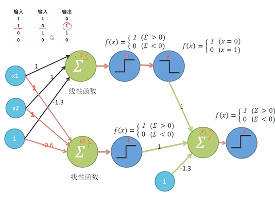
神经网络:主要用于分类和聚类
-
用一条线划分两种类型的属性---分割线计算
-
高维空间,只是变成了矩阵相乘---用面分割
-
神经元=激活函数=f(x)
-
手工拟合OR,AND,XOR
-
-
感知机:梯度下降实现
-
随便划线,感知点的情绪(- -),向着开心的方向进行移动
-
调整线的斜率,使结果更好
-
梯度下降:连续可导,可以求斜率
-
MSE最小均方差
-
Cross-entropy交叉熵
-
p(red)=p(blue)
-
sigmoid函数处理线性函数,
-
-
-
- 机器学习经典模型:KNN模型(人以类聚,物以群分)
-
聚类算法
-
相似的事务归为一类-标签化---物以类聚
- k-means
-
k:中心点的个数,质心
-
means:求平均
-
不断迭代,更新质心
-
步骤
-
1.选择聚类的个数K
-
2.生成K个聚类中心点
-
3.计算所有样本点到聚类中心点的距离
-
4.更新质心(求聚类后的x,y平均值),迭代聚类
-
5.重复4直到满足收敛要求
-
-
-
import numpy as np
import matplotlib.pyplot as plt
from sklearn.cluster import MiniBatchKMeans, KMeans
# 测量
from sklearn import metrics
# 球状簇
from sklearn.datasets.samples_generator import make_blobs

# 生成数据集,样本数=1000,特征数=2,中心=以哪些点为中心生成样本点,标准差=围绕中心的标准差,随机状态值=每次运行生成散点图一致
x, y = make_blobs(n_samples=1000, n_features=2, centers=([-1, -1], [0, 0], [1, 1], [2, 2]),
				  cluster_std=(0.4, 0.2, 0.2, 0.2), random_state=9)
# 生成散点图
plt.scatter(x[:, 0], x[:, 1], marker="o")
plt.show()

# 可视化
for index, k in enumerate((2, 3, 4, 5)):
	plt.subplot(2, 2, index + 1)
	# 随机选取200个点,分别用特征2,3,4,5作为特征值,进行K——means
	y_pred = MiniBatchKMeans(n_clusters=k, batch_size=200, random_state=9).fit_predict(x)
	# 聚类效果评分
	score = metrics.calinski_harabaz_score(x, y_pred)
	plt.scatter(x[:, 0], x[:, 1], c=y_pred)
	plt.text(.99,.01,
			 ('k=%d,score:%.2f' % (k, score)),
			 fontsize=10,
			 transform=plt.gca().transAxes,
			 horizontalalignment="right")
plt.show()
-
-
-
-
-
完整的预处理例子
-
'''
完整的机器学习流程
'''

# 1.导入库
import numpy as np
import pandas as pd
import matplotlib.pyplot as plt
import seaborn as sns
import numpy.random as nr
import math
from sklearn.cluster import MiniBatchKMeans, KMeans
# 测量
from sklearn import metrics
# 球状簇
from sklearn.datasets.samples_generator import make_blobs


# 2.观察数据集
# 路径带中文,前面先用open打开
auto_prices = pd.read_csv(open('工业汽车数据集应用实践/Automobile price data _Raw_.csv'))
# print(auto_prices.head(20))

# 3.数据的预处理,重新编码
auto_prices.columns = (str.replace('-', '_') for str in auto_prices.columns)

# 4.处理缺失值
# 找出所有缺失值
(auto_prices.astype(np.object) == '?').any()

for col in auto_prices.columns:
	if auto_prices[col].dtypes == object:
		count = 0
		count = [count + 1 for x in auto_prices[col] if x == '?']
		print(col + '	' + str(sum(count)))

# 处理缺失值
auto_prices.drop('normalized_losses', axis=1, inplace=True)
cols = ['price', 'bore', 'stroke', 'horsepower', 'peak_rpm']
for column in cols:
	auto_prices.loc[auto_prices[column] == '?', column] = np.nan
auto_prices.dropna(axis=0, inplace=True)
print(auto_prices.shape)

# 5.转换列数据类型
for column in cols:
	auto_prices[column] = pd.to_numeric(auto_prices[column])
print(auto_prices[cols].dtypes)

# 6.特征工程
# 汇总变量类别,转换ln,交互的变量合并
# 聚合特征变量
print(auto_prices['num_of_cylinders'].value_counts())
# print(auto_prices.columns)

cylinder_categories = {
	'three': 'three_four',
	'four': 'three_four',
	'five': 'five_six',
	'six': 'five_six',
	'eight': 'eight_twelve',
	'twelve': 'eight_twelve', }
auto_prices['num_of_cylinders'] = [cylinder_categories[x] for x in auto_prices['num_of_cylinders']]
print(auto_prices['num_of_cylinders'].value_counts())


# 7.箱型图
# 哪个特征影响价格走向
def plot_box(auto_price, col, col_y='price'):
	sns.set_style('whitegrid')
	sns.boxplot(col, col_y, data=auto_price)
	plt.xlabel(col)
	plt.ylabel(col_y)
	plt.show()


plot_box(auto_prices, 'num_of_cylinders')

print(auto_prices['body_style'].value_counts())
body_cats = {
	'sedan': 'sedan',
	'hatchback': 'hatchback',
	'wagon': 'wagon',
	'hardtop': 'hardtop_convert',
	'convertible': 'hardtop_convert', }
auto_prices['body_style'] = [body_cats[x] for x in auto_prices['body_style']]
print(auto_prices['body_style'].value_counts())


# 8.特征图
# 哪个特征有别于其他特征
def plot_box(auto_price, col, col_y='price'):
	sns.set_style('whitegrid')
	sns.boxplot(col, col_y, data=auto_price)
	plt.xlabel(col)
	plt.ylabel(col_y)
	plt.show()


plot_box(auto_prices, 'body_style')


# 9.转换变量
def hist_plot(vals, lab):
	sns.distplot(vals)
	plt.title('Histogram of' + lab)
	plt.xlabel('value')
	plt.ylabel('Density')
	plt.show()


hist_plot(auto_prices['price'], 'prices')
# 对数转换
auto_prices['log_price'] = np.log(auto_prices['price'])
hist_plot(auto_prices['log_price'], 'log_price')


# 10.可视化
# 看价格与其他特征是否存在线性或非线性的关系
def plot_scatter_shape(auto_prices, cols, shape_col='fuel_type', col_y='log_price', alpha=0.2):
	shapes = ['+', 'o', 's', 'x', '^']
	unique_cats = auto_prices[shape_col].unique()
	for col in cols:
		sns.set_style('whitegrid')
		for i, cat in enumerate(unique_cats):
			temp = auto_prices[auto_prices[shape_col] == cat]
			sns.regplot(col, col_y, data=temp, marker=shapes[i], label=cat,
						scatter_kws={'alpha': alpha}, fit_reg=False, color='blue')

		plt.title('scatter plot of' + col_y + 'vs.' + col)
		plt.xlabel(col)
		plt.ylabel(col_y)
		plt.legend()
		plt.show()


num_cols = ['curb_weight', 'engine_size', 'horsepower', 'city_mpg']
plot_scatter_shape(auto_prices, num_cols)
-
-
-
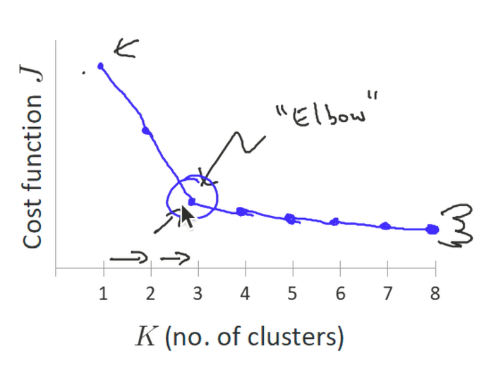
算法效果的衡量标准
-
SSE(Sum of Squear due to Error)误差平方和
- 每个点跟质心的距离
-
K值确定:Elbow method 肘方法
- SSE跟聚类个数画图
- 找出拐点来确定聚类数
- 轮廓系数法(Silhouette Coefficient)
- 根据轮廓边缘的变化感知聚类的凝聚度和分离度

-
CH(Calinski-Harabasz)
-
数据类别距离平方和越小越好,类别之间平方和越大越好
-

-
-
-