1 感知机

“知错能改”算法梗概：

目标：w1x1+w2x2=0是一条经过原点的直线，找到合适的参数w1,w2使得该直线的较好的区分两组数据

随机初始化参数w1,w2. 之前的法向量为(w1, w2)
开始迭代:
- 当对某一个数据错误的分类后，对两个参数w1, w2进行更新，(w1, w2).T是直线的法向量
- 具体的更新方法为 (new_w1, new_w2).T = (w1, w2).T + label * (x1, x2).T。即当
- 当所有的数据分类都正确时退出

算法演示

上面的动图中：

粉红与紫色的分界线被认为是寻找的直线
w(t)代表之前直线的法向量，w(t+1)表示更新得到的法向量
黑色标记表示当前直线下分类错误的点

import numpy as np
import matplotlib.pyplot as plt
%matplotlib inline

# 设置随机种子
np.random.seed(325)

# 随机生成o数据
o_data_x = np.random.randint(40, 80, 5)
o_data_y = np.random.randint(20, 80, 5)
o_label = np.array([1,1,1,1,1])

# 随机生成x数据
x_data_x = np.random.randint(10, 50, 5)
x_data_y = np.random.randint(60, 90, 5)
x_label = np.array([-1,-1,-1,-1,-1])

# 随机生成初始直线法向量
w1_w2 = np.random.random(2)
w1_w2

array([0.37665966, 0.86833482])

def plot(w1_w2, time):
    """
    画图函数
    
    parametes:
    1. w1_w2 --- numpy.ndarray类型，shape:(2,)，意为直线的法向量
    2. time --- int类型，意为第几次更新，初始值为0
    """
    # 设置画布
    plt.figure(figsize=(8, 8))
    plt.xlim([-110, 110])
    plt.ylim([-110, 110])

    # 作点
    plt.scatter(o_data_x, o_data_y, c='b', marker='o', label=' 1')
    plt.scatter(x_data_x, x_data_y, c='r', marker='x', label='-1')
    plt.legend(loc='upper left')

    # 作初始线
    t = np.linspace(-100, 100, 18)
    plt.plot(t, -w1_w2[0]/w1_w2[1]*t)

    # 获取当前的坐标轴, gca = get current axis
    ax = plt.gca()

    # 设置标题，也可用plt.title()设置
    if time == 0:
        title_name = 'Inital'
    elif time == 1:
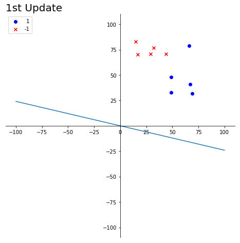
        title_name = '1st Update'
    elif time == 2:
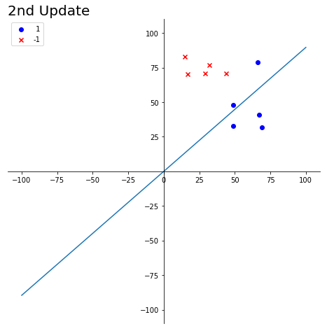
        title_name = '2nd Update'
    elif time == 3:
        title_name = '3rd Update'
    else:
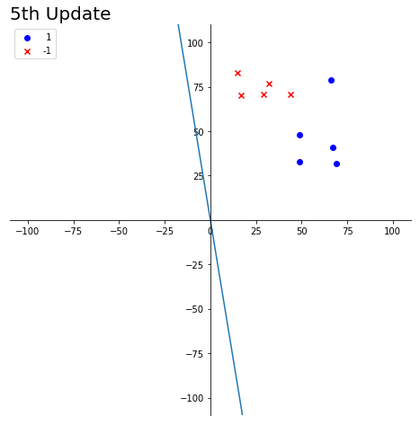
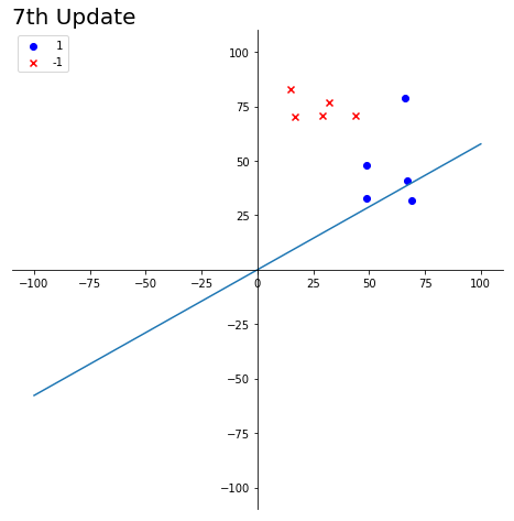
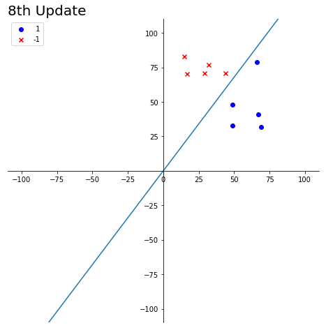
        title_name = str(time) + 'th Update'
    ax.set_title(title_name, fontsize=20, loc='left')
    
    # 设置右边框和上边框，隐藏
    ax.spines['right'].set_color('none')
    ax.spines['top'].set_color('none')

    # 设置x坐标轴为下边框，设置y坐标轴为左边框
    ax.xaxis.set_ticks_position('bottom')
    ax.yaxis.set_ticks_position('left')

    # 设置下边框, 左边框在(0, 0)的位置
    ax.spines['bottom'].set_position(('data', 0))
    ax.spines['left'].set_position(('data', 0))

    # 设置刻度
    ax.set_xticks([-100, -75, -50, -25, 0, 25, 50, 75, 100])
    ax.set_yticks([-100, -75, -50, -25, 25, 50, 75, 100])
    
    # 保存图片
    print("w1_w2 = ", w1_w2)
    plt.savefig(title_name + '.jpg')

# 初始态
plot(w1_w2, 0)

w1_w2 =  [0.37665966 0.86833482]

# 整合数据
train_X = np.vstack((np.hstack((o_data_x, x_data_x)),np.hstack((o_data_y, x_data_y))))
train_y = np.hstack((o_label, x_label))

# 转置
train_X = train_X.T

# 查看数据
print("train_x:
{0}
train_y:
{1}".format(train_X, train_y))

train_x:
[[49 33]
 [49 48]
 [67 41]
 [66 79]
 [69 32]
 [17 70]
 [15 83]
 [29 71]
 [44 71]
 [32 77]]
train_y:
[ 1  1  1  1  1 -1 -1 -1 -1 -1]

# 迭代更新
cnt = 0
while True:
    result = np.sign(np.dot(train_X, w1_w2))
    # 已经能够正确分类了
    if (result == train_y).all():
        break
    else:
    # 找到不能正确分类的那些数据并更新W1_w2
        for i in range(train_X.size):
            if result[i] != train_y[i]:
                w1_w2 += train_X[i] * train_y[i]
                cnt += 1
                plot(w1_w2, cnt)
                break

w1_w2 =  [-16.62334034 -69.13166518]
w1_w2 =  [ 32.37665966 -36.13166518]
w1_w2 =  [81.37665966 11.86833482]
w1_w2 =  [ 64.37665966 -58.13166518]
w1_w2 =  [130.37665966  20.86833482]
w1_w2 =  [113.37665966 -49.13166518]
w1_w2 =  [  69.37665966 -120.13166518]
w1_w2 =  [118.37665966 -87.13166518]