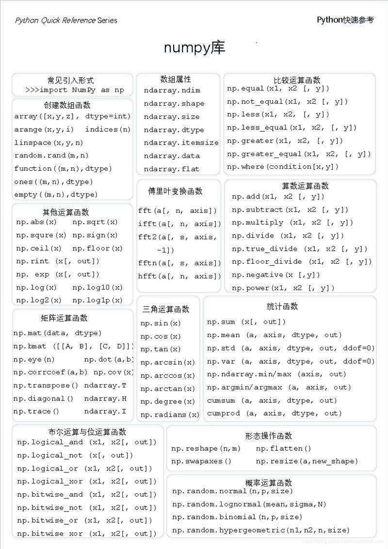
一、numpy库的学习总计
二、numpy的安装
安装方式I
安装numpy库
打开cmd命令行,输入:python3 -m pip install -U pip更新pip
pip install numpy 安装
安装方式II
pip install ipython
ipython –pylab
pylab模式下会自动导入SciPy,NumPy,Matplotlib模块
二、引入numpy
import numpy as py
使用numpy
arange() 函数用于创建同类型多维数组(homogeneous multidimensional array)
用arange创建的数组使用type()查看类型为ndarray
reshape() 函数用于重新构造数组成为其他维度数组
例如:np.arange(20).reshape(4,5)
[[ 0 1 2 3 4]
[ 5 6 7 8 9]
[10 11 12 13 14]
[15 16 17 18 19]]
arrry 数组相关属性:
ndim: 维度
shape: 各维度大小
size: 元素个数
dtype: 元素类型
dsize: 元素占位大小
生成特殊矩阵
全零矩阵:np.zeros()
注意:ones()和zeros()函数的第一个参数是一个指向数列的指针,不能直接是一个数列,例如上图报错情况
全一矩阵:np.ones(d,dtype=int)
默认生成浮点型,可通过第二个参数指定元素数据类型
1.随机数数组
np.random.rand(5)生成包含5个[0,1)区间的数的数组
2.数组计算
a = np.array([1.0, 2],[2, 4])
a
[[ 1. 2.]
[ 2. 4.]]
由于数组是【同质】的,python会自动将整型转换为浮点型
np.exp(a): 自然常数e(约等于2.7)的a次方
np.sqrt(a): a的开方
np.square(a):a的平方
np.power(a,3):a的3次方
a.sum(): 所有元素之和
a.max(): 最大元素
a.min(): 最小元素
a.max(axis=1): 每行最大
a.min(axis=0): 每列最小
数组与矩阵(matrix)
注意:
矩阵是二维数组,矩阵乘法相求左侧矩阵列数等于右侧矩阵行数
数组可以是任意正整数维数,乘法要求两侧数组行列数均相同
相互转换
3.数组转矩阵
np.asmatrix(a)
np.mat(a)
4.直接生成
np.matrix(‘1.0 2.0;3.0 4.0’)
5.生成指定长度的一维数组
np.linspace(0,2,9):生成从0开始,到2结束,包含9个元素的等差数列
6.数组元素访问
a = np.array([3.2, 1.5],[2.5, 4])
print a[0][1]
1.5
print a[0,1]
1.5
注意:
若b=a是将b和a同时指向同一个array,若修改a或者b的某个元素,a和b都会改变
若想a和b不会关联修改,则需要b = a.copy()为b单独生成一份拷贝
a:
[[ 0 1 2 3 4]
[ 5 6 7 8 9]
[10 11 12 13 14]
[15 16 17 18 19]]
a[: , [1,3]]:访问a的所有行的2、4列
**访问符合条件的元素
a[: , 2][a[: , 0] > 5]
解释:
a [x] [y]表示访问符合x、y条件的a的元素,[: , 2]表示取所有行的第3列,[a[: , 0] > 5]表示取第一列大于5的行(即第3、4行),最终即表示取第3、4行的第3列,即得结果array([12, 17])这个“子”数组
numpy.where()查找符合条件的位置
例如:loc = np.where(a == 11)
print loc
(array([2]), array([1]))
结果是一个表示坐标的元组,元组第一个数组表示查询结果的行坐标,第二个数组表示结果的列坐标
print a[loc[0][0], loc[1][0]]
11
上式为通过位置反求元素11
注意:where求出的结果为元组,不能通过loc[x,y]的方式获取元素(该获取方式为数组的方式,因为元组没有索引),只能通过loc[x][y]的方式获取
7.数组其他操作
矩阵转置
a = np.random.rand(2,4)
a = np.transpose(a)将a数组转置
b = np.random.rand(2,4)
b = np.mat(b)
print b.T 转置矩阵
矩阵求逆
import numpy.linalg as nlg
a = np.random.rand(2,2)
a = np.mat(a)
ia = nlg.inv(a) 得逆矩阵
print a * ia
[[ 1. 0.]
[ 0. 1.]]
特征值和特征向量
a = np.random.rand(3,3)
eig_value, eig_vector = nlg.eig(a)
拼接矩阵(使用场景:循环处理某些数据后的操作)
按列拼接两个向量成一个矩阵
vstack
hstack
实例:
1 a = np.random.rand(2,2)
2 b = np.random.rand(2,2)
3 c = np.hstack([a,b]) 水平拼接
4 d = np.vstack([a,b]) 垂直拼接
缺失值
nan作为缺失值的记录
通过isnan判定
a = np.random.rand(2,2)
a[0, 1] = np.nan
print (np.isnan(a))
nan_to_num可用来将nan替换成0
pandas提供能指定nan替换值的函数
print(np.nan_to_num(a))
[[ 0.54266589 0.46546544 ]
[ 0.92468339 0.70599254]]
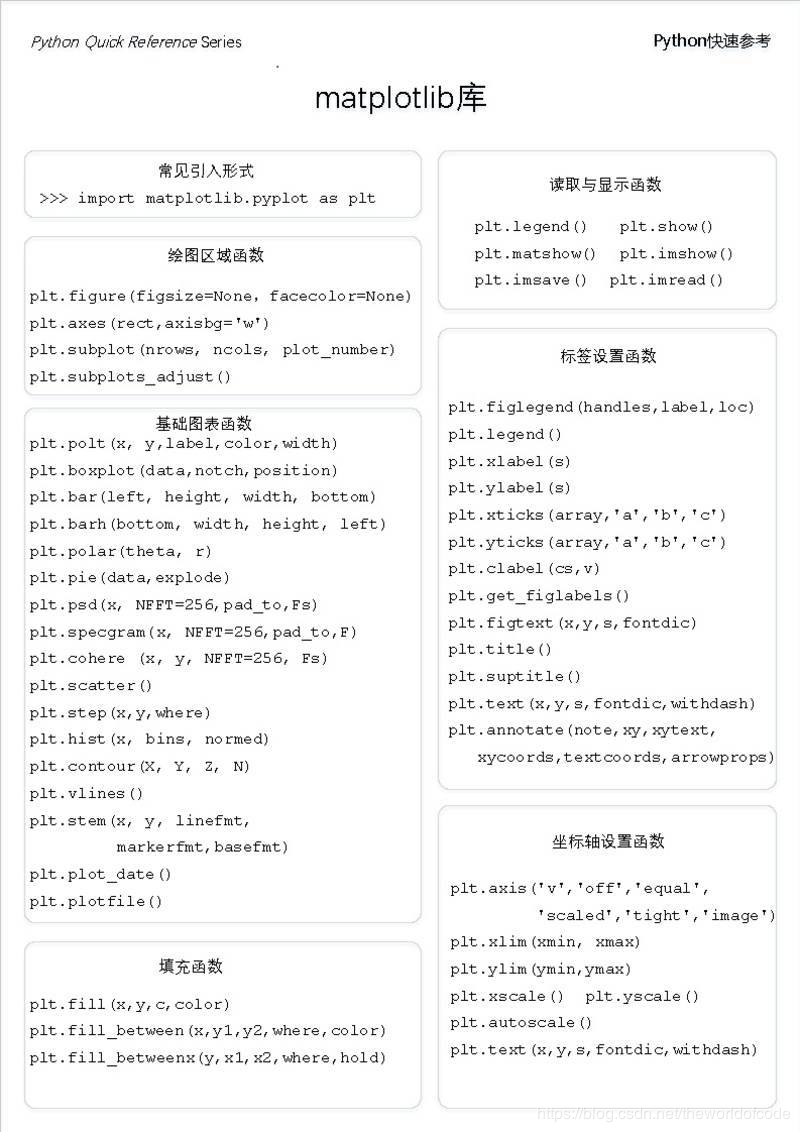
三、matplotlib的学习总结
实例1:基本三角函数图像实现
1 import numpy as np
2 import matplotlib.pyplot as plt
3 x = np.linspace(0, 6, 100)
4 y = np.cos(2 * np.pi * x) * np.exp(-x)+0.8
5 plt.plot(x, y, 'k', color='r', linewidth=3, linestyle="-")
6 plt.show()

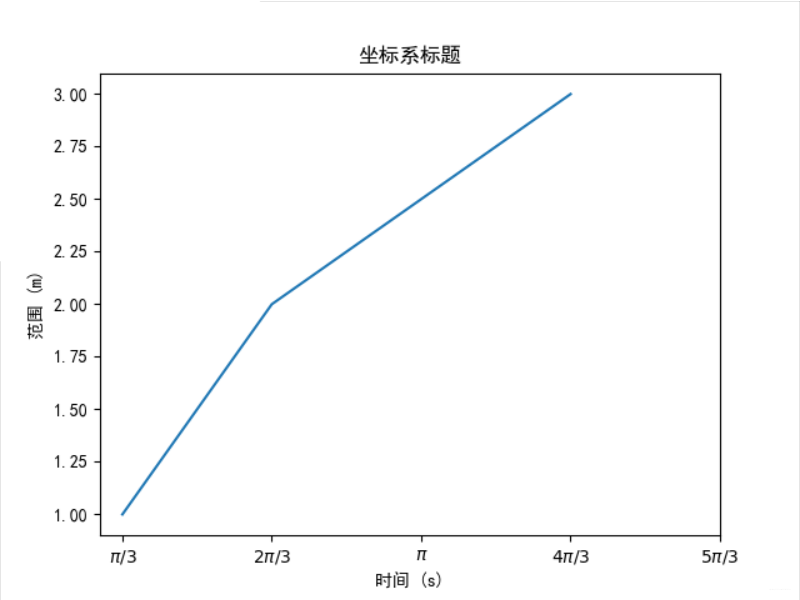
 1 import matplotlib.pyplot as plt
 2 import matplotlib
 3 matplotlib.rcParams['font.family']='SimHei'
 4 matplotlib.rcParams['font.sans-serif'] = ['SimHei']
 5 plt.plot([1,2,4], [1,2,3])
 6 plt.title("坐标系标题")
 7 plt.xlabel('时间 (s)')
 8 plt.ylabel('范围 (m)')
 9 plt.xticks([1,2,3,4,5],[r'$pi/3$', r'$2pi/3$', r'$pi$',
10                    r'$4pi/3$', r'$5pi/3$'])
11 plt.show()
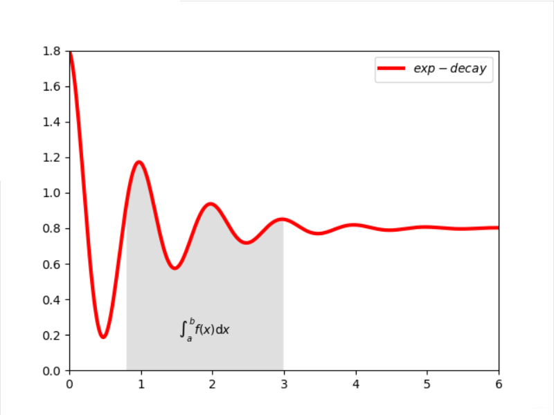
实例2:带标识的坐标系
 1 import matplotlib.pyplot as plt
 2 import numpy as np
 3 x = np.linspace(0, 10, 1000)
 4 y = np.cos(2*np.pi*x) * np.exp(-x)+0.8
 5 plt.plot(x,y,'k',color='r',label="$exp-decay$",linewidth=3)
 6 plt.axis([0,6,0,1.8])
 7 ix = (x>0.8) & (x<3)
 8 plt.fill_between(x, y ,0, where = ix,
 9                          facecolor='grey', alpha=0.25)
10 plt.text(0.5*(0.8+3), 0.2, r"$int_a^b f(x)mathrm{d}x$",
11                 horizontalalignment='center')
12 plt.legend()
13 plt.show()
实例3:带阴影的坐标系
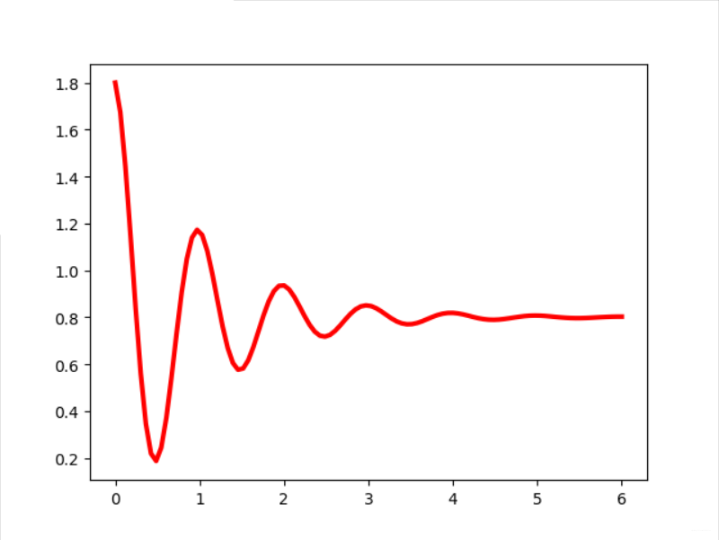
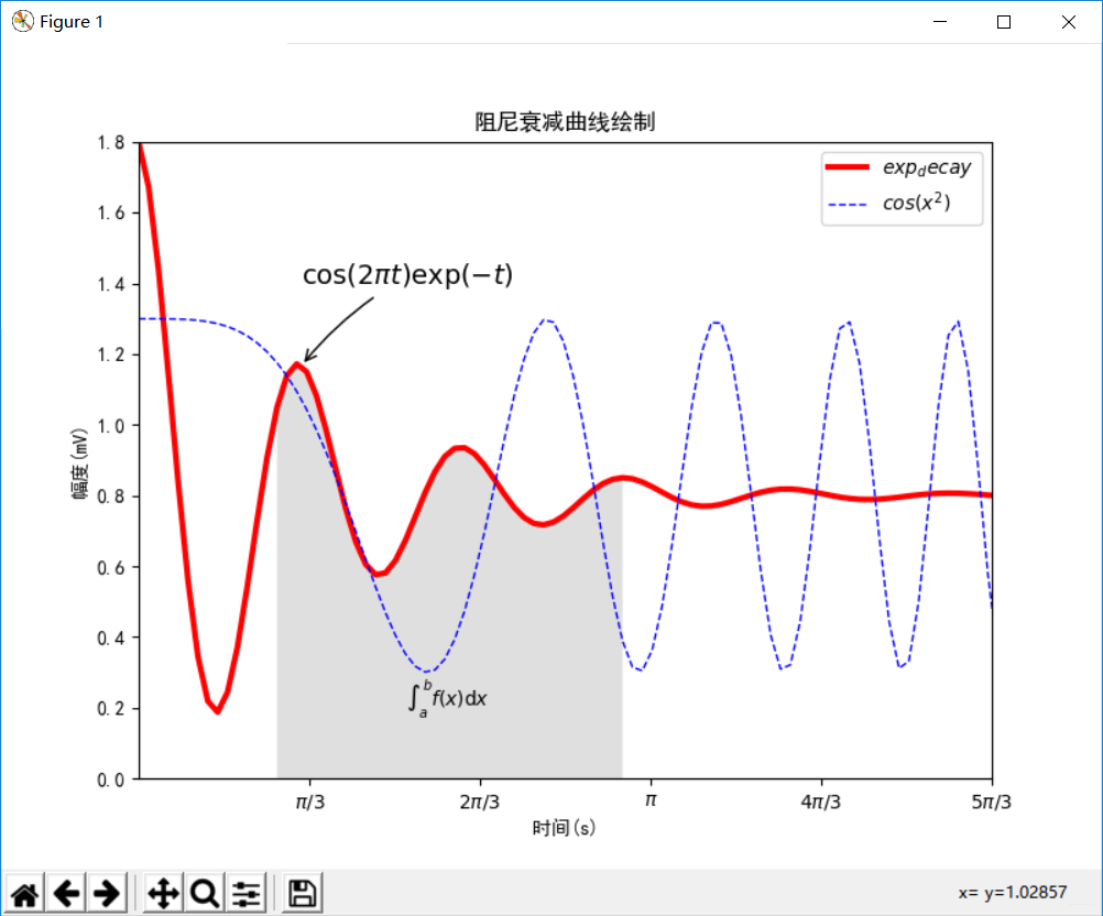
实例4:带阻尼衰减曲线坐标图绘制
 1 ##e18.1PlotDamping.py
 2 import numpy as np
 3 import matplotlib.pyplot as plt
 4 import matplotlib
 5 matplotlib.rcParams['font.family']='SimHei'
 6 matplotlib.rcParams['font.sans-serif'] = ['SimHei']
 7 def Draw(pcolor, nt_point, nt_text, nt_size):
 8     plt.plot(x, y, 'k', label="$exp_decay$", color=pcolor, linewidth=3, linestyle="-")
 9     plt.plot(x, z, "b--", label="$cos(x^2)$", linewidth=1)
10     plt.xlabel('时间(s)')
11     plt.ylabel('幅度(mV)')
12     plt.title("阻尼衰减曲线绘制")
13     plt.annotate('$cos(2 pi t) exp(-t)$', xy=nt_point, xytext=nt_text, fontsize=nt_size,
14                arrowprops=dict(arrowstyle='->', connectionstyle="arc3,rad=.1"))
15 def Shadow(a, b):
16     ix = (x>a) & (x<b)
17     plt.fill_between(x,y,0,where=ix,facecolor='grey', alpha=0.25)
18     plt.text(0.5 * (a + b), 0.2, "$int_a^b f(x)mathrm{d}x$",
19              horizontalalignment='center')
20 def XY_Axis(x_start, x_end, y_start, y_end):
21     plt.xlim(x_start, x_end)
22     plt.ylim(y_start, y_end)
23     plt.xticks([np.pi/3, 2 * np.pi/3, 1 * np.pi, 4 * np.pi/3, 5 * np.pi/3],
24                ['$pi/3$', '$2pi/3$', '$pi$', '$4pi/3$', '$5pi/3$'])
25 x = np.linspace(0.0, 6.0, 100)
26 y = np.cos(2 * np.pi * x) * np.exp(-x)+0.8
27 z = 0.5 * np.cos(x ** 2)+0.8
28 note_point,note_text,note_size = (1, np.cos(2 * np.pi) * np.exp(-1)+0.8),(1, 1.4), 14
29 fig = plt.figure(figsize=(8, 6), facecolor="white")
30 plt.subplot(111)
31 Draw("red", note_point, note_text, note_size)
32 XY_Axis(0, 5, 0, 1.8)
33 Shadow(0.8, 3)
34 plt.legend()
35 plt.savefig('sample.JPG')
36 plt.show()
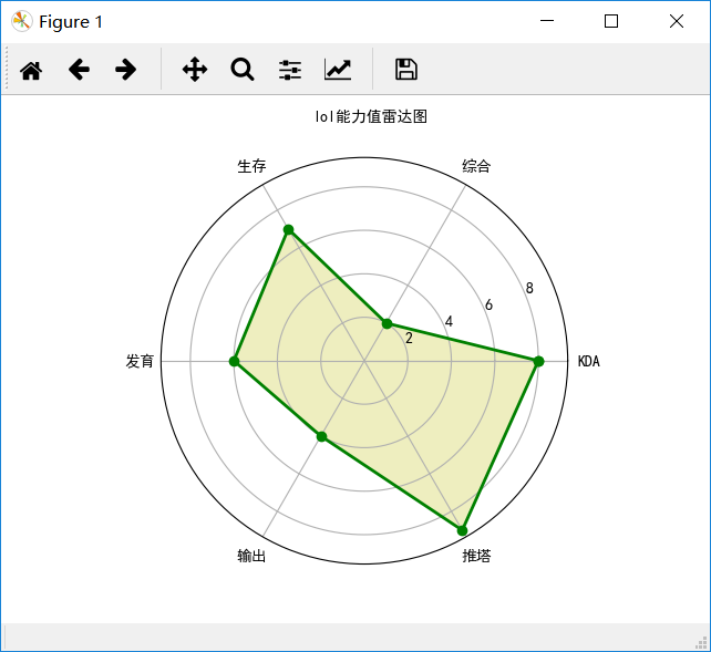
实例五多级雷达图绘制
lol人物能力值雷达图绘制
代码如下:
 1 # -*- coding: utf-8 -*-
 2 ##e19.1DrawRadar
 3 import numpy as np
 4 import matplotlib.pyplot as plt
 5 import matplotlib
 6 matplotlib.rcParams['font.family']='SimHei'
 7 matplotlib.rcParams['font.sans-serif'] = ['SimHei']
 8 labels = np.array(['KDA', '综合', '生存', '发育', '输出', '推塔'])
 9 nAttr = 6
10 data = np.array([8, 2, 7, 6, 4, 9]) #数据值
11 angles = np.linspace(0, 2*np.pi, nAttr, endpoint=False)
12 data = np.concatenate((data, [data[0]]))
13 angles = np.concatenate((angles, [angles[0]]))
14 fig = plt.figure(facecolor="white")
15 plt.subplot(111, polar=True)
16 plt.plot(angles,data,'bo-',color ='g',linewidth=2)
17 plt.fill(angles,data,facecolor='y',alpha=0.25)
18 plt.thetagrids(angles*180/np.pi, labels)
19 plt.figtext(0.52, 0.95, 'lol能力值雷达图', ha='center')
20 plt.grid(True)
21 plt.show()
效果图如下:
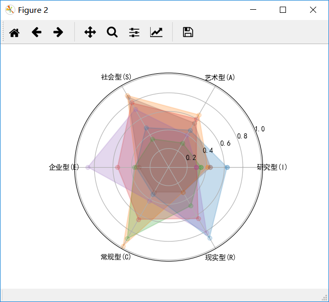
实例6:霍兰德人格分析雷达图绘制
 1 #e19.2DrawHollandRadar
 2 import numpy as np
 3 import matplotlib.pyplot as plt
 4 import matplotlib
 5 matplotlib.rcParams['font.family']='SimHei'
 6 matplotlib.rcParams['font.sans-serif'] = ['SimHei']
 7 radar_labels = np.array(['研究型(I)','艺术型(A)','社会型(S)','企业型(E)','常规型(C)','现实型(R)'])
 8 nAttr = 6
 9 data = np.array([[0.63, 0.42, 0.35, 0.30, 0.30, 0.45],
10                  [0.46, 0.65, 0.30, 0.60, 0.40, 0.55],
11                  [0.49, 0.89, 0.35, 0.80, 0.72, 0.87],
12                  [0.35, 0.35, 0.37, 0.55, 0.87, 0.32],
13                  [0.34, 0.98, 0.89, 0.65, 0.42, 0.31],
14                  [0.88, 0.31, 0.48, 0.64, 0.82, 0.31]]) #数据值
15 data_labels = ('工程师', '实验员', '艺术家', '推销员', '社会工作者','记事员')
16 angles = np.linspace(0, 2*np.pi, nAttr, endpoint=False)
17 data = np.concatenate((data, [data[0]]))
18 angles = np.concatenate((angles, [angles[0]]))
19 fig = plt.figure(facecolor="white")
20 plt.subplot(111, polar=True)
21 #plt.plot(angles,data,'bo-',color ='gray',linewidth=1,alpha=0.2)
22 plt.plot(angles,data,'o-', linewidth=1.5, alpha=0.2)
23 plt.fill(angles,data, alpha=0.25)
24 plt.thetagrids(angles*180/np.pi, radar_labels,frac = 1.2)
25 plt.figtext(0.52, 0.95, '霍兰德人格分析', ha='center', size=20)
26 legend = plt.legend(data_labels, loc=(0.94, 0.80), labelspacing=0.1)
27 plt.setp(legend.get_texts(), fontsize='small')
28 plt.grid(True)
29 plt.show()
效果图如下所示:
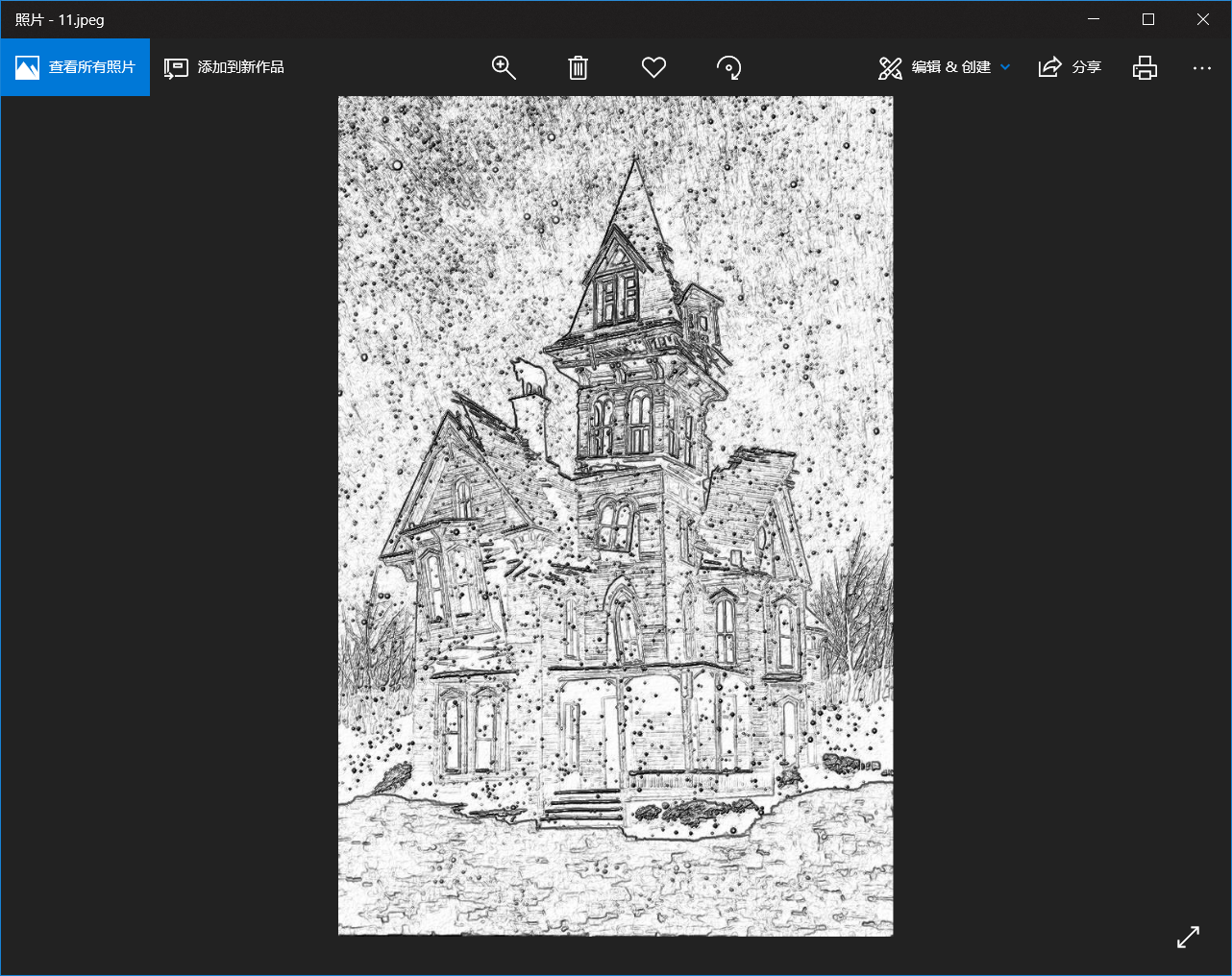
四、自定义手绘风
代码如下:
 1 #e17.1HandDrawPic.py
 2 from PIL import Image
 3 import numpy as np
 4 vec_el = np.pi/2.2 # 光源的俯视角度,弧度值
 5 vec_az = np.pi/4. # 光源的方位角度,弧度值
 6 depth = 10. # (0-100)
 7 im = Image.open('E:\111.jpeg').convert('L')
 8 a = np.asarray(im).astype('float')
 9 grad = np.gradient(a) #取图像灰度的梯度值
10 grad_x, grad_y = grad #分别取横纵图像梯度值
11 grad_x = grad_x*depth/100.
12 grad_y = grad_y*depth/100.
13 dx = np.cos(vec_el)*np.cos(vec_az) #光源对x 轴的影响
14 dy = np.cos(vec_el)*np.sin(vec_az) #光源对y 轴的影响
15 dz = np.sin(vec_el) #光源对z 轴的影响
16 A = np.sqrt(grad_x**2 + grad_y**2 + 1.)
17 uni_x = grad_x/A
18 uni_y = grad_y/A
19 uni_z = 1./A
20 a2 = 255*(dx*uni_x + dy*uni_y + dz*uni_z) #光源归一化
21 a2 = a2.clip(0,255)
22 im2 = Image.fromarray(a2.astype('uint8')) #重构图像
23 im2.save('E:\11.jpeg')
原图:

效果图:
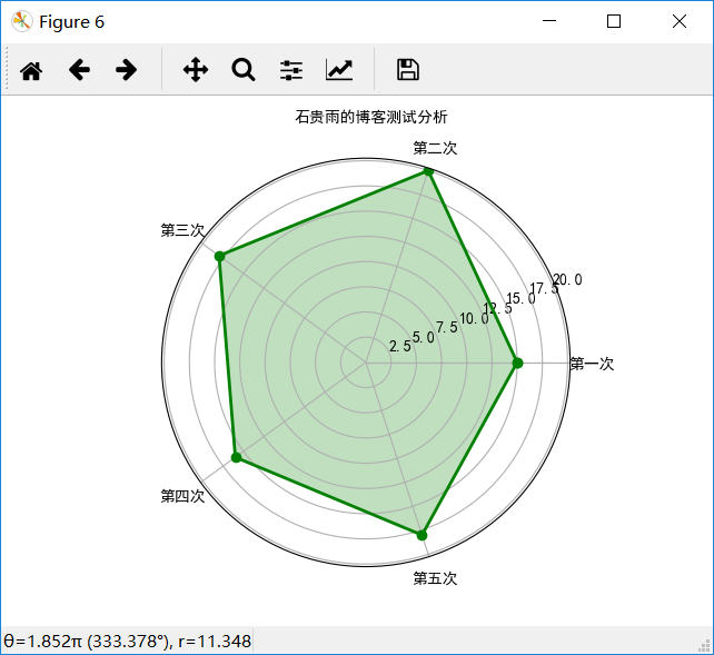
五、模仿实例对自己的成绩进行分析
代码如下:
 1 import numpy as np
 2 import matplotlib.pyplot as plt
 3 import matplotlib
 4 matplotlib.rcParams['font.family']='SimHei'
 5 matplotlib.rcParams['font.sans-serif'] = ['SimHei']
 6 labels = np.array(['第一次', '第二次', '第三次', '第四次', '第五次'])
 7 nAttr = 5
 8 data = np.array([15,20,18,16,18]) #数据值
 9 angles = np.linspace(0, 2*np.pi, nAttr, endpoint=False)
10 data = np.concatenate((data, [data[0]]))
11 angles = np.concatenate((angles, [angles[0]]))
12 fig = plt.figure(facecolor="white")
13 plt.subplot(111, polar=True)
14 plt.plot(angles,data,'bo-',color ='g',linewidth=2)
15 plt.fill(angles,data,facecolor='g',alpha=0.25)
16 plt.thetagrids(angles*180/np.pi, labels)
17 plt.figtext(0.52, 0.95, '石贵雨的博客测试分析', ha='center')
18 plt.grid(True)
19 plt.show()
效果图如下: