图像分割算法初探 彩英

       图像分割是计算机视觉研究中的一个经典难题，已经成为图像理解领域的一个热点。图像分割是图像分析的第一步，是计算机视觉的基础和图像理解的重要组成部分，同时也是图像处理中最困难的问题之一。所谓图像分割，是指根据灰度、空间纹理、几何形状等特征把图像划分成若干个互不相交的区域，使得这些特征在同一区域内表现出一致性或相似性，而在不同区域间表现出出明显的不同。简单来说，就是在一幅图像中，把目标从背景中分离出来。虽然到目前为止，还不存在一个完美通用的图像分割的方法，但也已经产生相当多的研究成果和方法。

       在深度学习大火之前，人们利用数字图像处理、拓扑学、数学等方面的知识来进行图像分割。随着算力的增加和深度学习的不断发展，一些传统分割算法在效果上已经不能与基于深度学习的分割算法相比较了，但传统图像分割的一些思想和技巧仍然值得我们借鉴和学习。

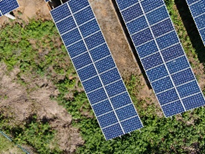
       下面介绍一种基于传统的图像处理技术的图像分割方法，即阈值分割方法。在此以光伏电板图像上的组件分割为例，简要说明以阈值分割为代表的图像处理方法的图像分割算法。光伏发电作为一种新能源发电方式，目前已经取得了广泛的应用。光伏电板在长期工作时，由于各种环境因素的影响，导致电板经常出现各种故障。因此，当使用成像设备拍摄光伏电板图像以观测其存在的故障时，首先要对图像进行分割，即将图像中每一个组件分割出来，确定每一个组件在图像中的位置，才能进一步对某一个存在故障的组件进行排查。

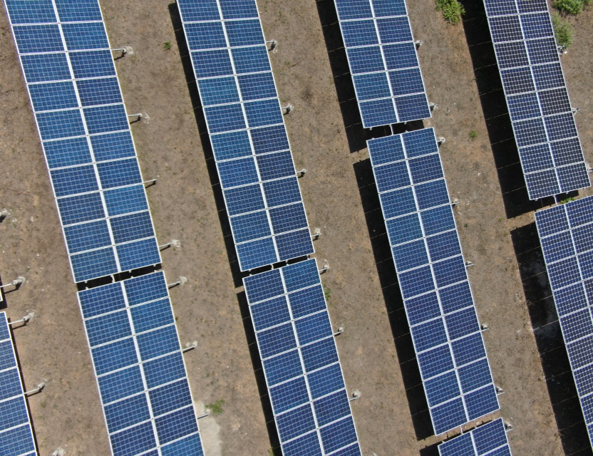
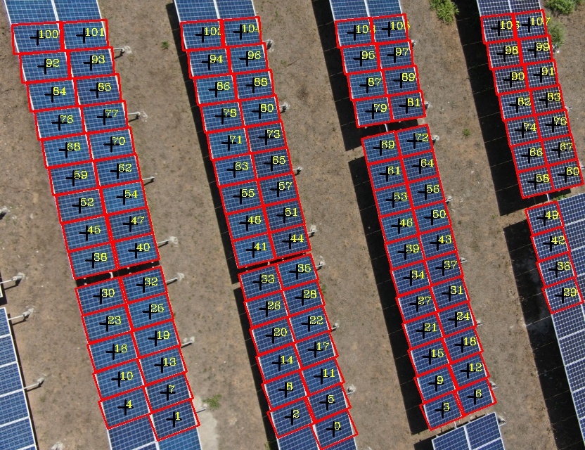
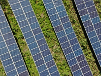
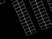
        以下面一组数据为例，说明图像分割的目的。左图为排列整齐的光伏电板的图像，右图为分割结果，分割结果图像中红色框框为每一个组件的边缘，每一个红色框框中的黑色十字为框框的中心位置标记，黄色数字为组件标号，图中组件的标号依次从0取到107，表示图中能够完整分割出来的组件一共有108个。

                                                     

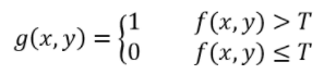
       上面右图中的分割结果是通过阈值分割实现的，那么阈值分割的原理是如何的呢？对于一幅图像，若这副图像由亮的目标和深的背景组成，则可利用目标和背景之间的灰度值的差异，将一整幅图像中的目标和背景分离开来。从背景中提取对象的一种显然的方法是选择一个阈值T，然后将所有的的点成为对象点，否则称其为背景点。该方法可用下面的公式表示：

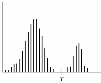
       若用直方图表示阈值分割的过程则更加清晰明了。如下图所示，如果目标区域的灰度值较大，而背景区域的灰度值较小，则图中所示的阈值T可将目标灰度值和背景灰度值分离出来，达到提取图像中目标的目的。

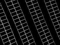
       以上面的光伏电板图像为例，图像中光伏电板组件的边缘较亮，即其灰度值较大，因此可设置一个较大的灰度值将组件的边缘分割出来。整幅图像的灰度值变化范围是0-255，此次实验过程中，将分割的阈值设置为140，即140-255区间范围内的灰度值设置为目标区域，可将其视作是组件的边缘。阈值分割的初始目标图像如下：

       对于上面的初始分割结果，应该使用OpenCV中的findContours函数去寻找组件的边缘，并使用框框将每一个组件框选出来。但是，如果你仔细观察该阈值分割的结果的话，会发现组件边缘之外存在许多噪声，即不是组件的目标的边缘也被分割了出来。因此，若直接使用findContours函数去寻找组件边缘，则容易将多余的边缘也使用边框框出来，这样就难以做到识别图像中组件的边缘了。

       从分割结果图像中很直观的感受来看，每一个组件之间的面积是差不多大小的，因此可以设置面积(边框长和宽的乘积)阈值，大致将组件挑选出来。面积阈值凭经验设置，本例中大概为1200-2500左右，使用面积阈值后的分割结果如下图所示：

        观察通过面积阈值过滤得到的组件边缘，发现已经可以基本上排除组件之外杂物对分割结果的影响了。但是，仍然有个别两个不是组件的边框也被画在了识别结果图像之中，这样也会造成组件边框识别的误判。为此，应该设置更多的条件，以过滤掉不符合实际但又被识别出来的边框。我们观察上图中识别到的边框，凡是组件的边框的话，会发现它们大小大致相等，而误判的边框的大小则和组件边框大小有较大差距。因此，可计算识别出的所有边框的长或者宽的平均标准差以衡量长或宽的离散程度，以长或宽的平均标准差的数值将所有组件的长或宽限制在一定范围内，从而排除识别边缘误判的情况。

       如果采用平均值标准差滤波的方法对误判的边缘进行滤波后，则可基本上排除误判的边缘了，下面给出最终识别组件边框的结果图像，发现其中没有一个组件边缘遗漏，也没有一个误判的边缘。对该边框识别结果的原始光伏电板图像中的组件进行边框标记，则可达到识别图像中所有组件的目的。

       上述基于阈值分割算法的代码如下给出，注意需要使用OpenCV:

#include <iostream>
#include <vector>
#include <string>

#include "opencv2/core/core.hpp"
#include "opencv2/highgui/highgui.hpp"
#include "opencv2/imgproc/imgproc.hpp"

using namespace std;
using namespace cv;

void threshold2(Mat gray, Mat& thresh, int minValue, int maxValue);
vector<vector<Point>> selectShapeArea(vector<vector<Point>> contours, int minValue, int maxValue);
vector<vector<Point>> vote(vector<vector<Point>> contours);
vector<vector<Point>> thetaFilter(vector<vector<Point>>& contours, vector<int>& filter_idx, int theta_range);
vector<vector<Point>> meanStdFilter(vector<vector<Point>>& contours, vector<int>& filter_idx, string& width_height, int n);

void threshold2(Mat gray, Mat& thresh, int minValue, int maxValue)
{
    Mat thresh1; Mat thresh2;
    threshold(gray, thresh1, minValue, 255, THRESH_BINARY);
    threshold(gray, thresh2, maxValue, 255, THRESH_BINARY_INV);
    thresh = thresh1 & thresh2;
}

vector<vector<Point>> selectShapeArea(vector<vector<Point>> contours, int minValue, int maxValue)
{
    vector<vector<Point>> result_contours;
    for (int i = 0; i < contours.size(); i++)
    {
        int contour_area = contourArea(contours[i]);
        if (contour_area > minValue && contour_area < maxValue)
        {
            result_contours.push_back(contours[i]);
        }
    }
    return result_contours;
}

vector<vector<Point>> vote(vector<vector<Point>> contours)
{
    int left = 0; int right = 0;
    vector<vector<Point>> leftcontours; 
    vector<vector<Point>> rightcontours;
    vector<vector<Point>> result;

    for (int i = 0; i < contours.size(); i++)
    {
        RotatedRect minRect = minAreaRect(Mat(contours[i]));
        float width = minRect.size.width; float height = minRect.size.height;

        if (width >= height)
        {
            leftcontours.push_back(contours[i]);
            left++;
        }
        else
        {
            rightcontours.push_back(contours[i]);
            right++;
        }
    }

    if (left >= right) result = leftcontours;
    else result = rightcontours;

    return result;
}

vector<vector<Point>> thetaFilter(vector<vector<Point>>& contours, vector<int>& filter_idx, int theta_range = 13)
{
    vector<vector<Point>> result;
    vector<int> _theta_table(180, 0);

    for (int i = 0; i < contours.size(); i++)
    {
        RotatedRect minRect = minAreaRect(Mat(contours[i]));
        int theta = (int)minRect.angle;

        for (int t = theta - theta_range; t <= theta + theta_range; t++)
        {
            if (t < 0) _theta_table[t + 180]++;
            else if (t >= 180) _theta_table[t - 180]++;
            else _theta_table[t]++;
        }
    }

    int inter_theta = max_element(_theta_table.begin(), _theta_table.end()) - _theta_table.begin();
    int l = find(_theta_table.begin(), _theta_table.end(), _theta_table[inter_theta]) - _theta_table.begin();
    int r = _theta_table.rend() - find(_theta_table.rbegin(), _theta_table.rend(), _theta_table[inter_theta]) - 1;
    int main_theta = (l + r) / 2;

    //cout << main_theta << endl;

    for (int i = 0; i < contours.size(); i++)
    {
        RotatedRect minRect = minAreaRect(Mat(contours[i]));
        int theta = (int)minRect.angle;

        if (theta < 0) theta = theta + 180;
        else if (theta >= 180) theta = theta - 180;
        else theta = theta;

        int distance = abs(theta - main_theta);
        //cout << distance << endl;
        if (distance <= theta_range || distance >= 180 - theta_range)
        {
            result.push_back(contours[i]);
        }
        else
        {
            filter_idx.push_back(i);
        }
    }
    return result;
}

vector<vector<Point>> meanStdFilter(vector<vector<Point>>& contours, vector<int>& filter_idx, string& width_height, int n = 3)
{
    vector<vector<Point>> result;
    result.reserve(contours.size());

    vector<float> data;

    for (int i = 0; i < contours.size(); i++)
    {
        RotatedRect minRect = minAreaRect(Mat(contours[i]));
        float width = minRect.size.width; float height = minRect.size.height;

        if (width_height == "width") data.push_back(width);
        else if (width_height == "height") data.push_back(height);
    }
   
    bool stop = false;
    vector<int> mask(data.size(), 1);
    int N = data.size();

    while (!stop)
    {
        float mean = 0.0; float std = 0.0;

        for (int i = 0; i < data.size(); i++)
        {
            if (mask[i] == 1) mean += data[i] / N;
        }

        for (int i = 0; i < data.size(); i++)
        {
            if (mask[i] == 1) std += (data[i] - mean) * (data[i] - mean) / N;
        }

        std = sqrt(std);
        float high = mean + n * std; float low = mean - n * std;
        stop = true;

        for (int i = 0; i < data.size(); i++)
        {
            if (low < data[i] && data[i] < high);
            else
            {
                if (mask[i] == 1)
                {
                    stop = false;
                    mask[i] = 0;
                    N--;
                }
            }
        }
    }

    for (int i = 0; i < contours.size(); i++)
    {
        if (mask[i] == 1) result.push_back(contours[i]);
        else filter_idx.push_back(i);
    }

    return result;
}

int main()
{
    //read the image
    Mat img = imread("the path for the picture");
    Mat bw; Mat gray; Mat edge;

    cvtColor(img, gray, COLOR_BGR2GRAY);
    imwrite("gray.jpg", gray);
 
    threshold2(gray, bw, 140, 255);
    imwrite("bw.jpg", bw);

    Mat bw_canny;
    Canny(bw, bw_canny, 100, 120, 3);
    imwrite("bw_canny.jpg", bw_canny);

    //morphology operation 
    Mat element = getStructuringElement(MORPH_ELLIPSE, Size(1, 1), Point(-1, -1));
    dilate(bw, bw, element, Point(-1, -1), 3);
    imwrite("dilate.jpg", bw);
    
    //find and draw contours
    vector<vector<Point>> contours;
    vector<Vec4i> hierarchy;
    findContours(bw, contours, hierarchy, CV_RETR_LIST, CV_CHAIN_APPROX_NONE);

    vector<vector<Point>> contours_area; 
    contours_area = selectShapeArea(contours, 1200, 2500);

    Mat bw_color = Mat::zeros(bw.rows, bw.cols, CV_8UC3);
    Mat bw_final = Mat::zeros(bw.rows, bw.cols, CV_8UC3);
    vector<Mat> channels(3);
    split(bw_color, channels);

    channels[2] = bw; channels[1] = bw; channels[0] = bw;
    merge(channels, bw_final);

    imwrite("middle.jpg", bw_final);

    vector<int> filter_idx;
    //vector<vector<Point>> contours_angle = thetaFilter(contours_area, filter_idx);
    //vector<vector<Point>> contours_final = vote(contours_angle);

    string wh_choose1 = "width"; string wh_choose2 = "height";

    vector<vector<Point>> contours_final = meanStdFilter(contours_area, filter_idx, wh_choose1);
    contours_final = meanStdFilter(contours_final, filter_idx, wh_choose2);

    for (int i = 0; i < contours_final.size(); i++)
    {
        RotatedRect minRect = minAreaRect(Mat(contours_final[i]));
        Point2f rect_points[4]; Point2f center_point; double rect_angle;
        minRect.points(rect_points);
        center_point = minRect.center;
        rect_angle = minRect.angle;

        double length = arcLength(contours_final[i], true);

        cout << "标号：" << i << "width：" << minRect.size.width << "height：" \
            << minRect.size.height << "length:" << length << endl << "angle:" << rect_angle << endl;

        double x0, y0;
        x0 = center_point.x;
        y0 = center_point.y;

        int w = 10; //十字叉的宽度                      
        //绘制轮廓的中心
        line(img, Point2f(x0 - w, y0), Point2f(x0 + w, y0), Scalar(0), 2);
        line(img, Point2f(x0, y0 - w), Point2f(x0, y0 + w), Scalar(0), 2);

        //设置绘制文本的相关参数
        string text = to_string(i);
        int font_face = FONT_HERSHEY_COMPLEX;
        double font_scale = 0.5;
        int thickness = 1;
        int baseline;

        putText(img, text, center_point, font_face, font_scale, Scalar(0, 255, 255), thickness, 8, 0);

        for (int j = 0; j < 4; j++)
        {
            line(img, rect_points[j], rect_points[(j + 1) % 4], Scalar(0, 0, 255), 2);
        }

        for (int j = 0; j < 4; j++)
        {
            line(bw_final, rect_points[j], rect_points[(j + 1) % 4], Scalar(0, 0, 255), 2);
        }
    }

    imwrite("img.jpg", img);
    imwrite("final.jpg", bw_final);

    waitKey(0);
    return 0;
}

        通过上面的实验，您也发现利用传统的图像处理技术对图像进行分割时，会有噪声的干扰、设定若干阈值等各种限制，这导致其无法在实际的工业生产等中得到很好的应用。而近年来深度学习的发展和广泛应用，则为图像分割创造了良好的工业应用的条件。下面依然以光伏电板图像分割为例，说明深度学习算法在图像分割中的广泛应用。

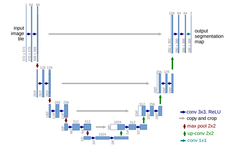
        在此介绍U-Net深度学习的方法对光伏电板图像进行分割，从而识别其中的组件边缘。关于U-Net的论文 "U-Net: Convolutional Networks for Biomedical Image Segmentation" 发表于2015年，最早应用于医疗影像中细胞图像的分割，属于语义分割的范围。语义分割(Semantic Segmentation)是图像处理和机器视觉的一个重要分支，与分类任务不同，语义分割需要判断图像每一个像素点的类别，进行精确分割。语义分割目前在自动驾驶，自动抠图和医疗影像等领域有着比较广泛的应用。U-Net是一种最常用和最简单的语义分割的模型，它简单、高效、易懂、容易构建且适用于小规模的数据集的训练。

        下图为U-Net的网络模型，整个网络如同字母U，简单来说，整个网络分为两个部分，左边部分负责特征提取，随着网络层加深，图像的通道数逐渐增加，而尺寸逐渐减小；右边的网络负责特征的还原，整个网络实际上就是一个编码解码器。需要注意的是，图中的灰色箭头部分，其表示将编码过程中得到的特征图像和解码过程中的特征图像进行合并的过程。在编码过程中，由于网络的最大值池化(Maxpooling)和二维卷积(Conv2D)作用，部分信息丢失。所以在解码时，需要在解码层的特征图像加入与之对应的编码层信息。

        实现上述U-Net网络结构的py代码如下：

import torch
from torch import nn
class DoubleConv(nn.Module):
    def __init__(self, in_ch, out_ch):
        super(DoubleConv, self).__init__()
        self.conv = nn.Sequential(
            nn.Conv2d(in_ch, out_ch, 3, padding=1),
            nn.BatchNorm2d(out_ch),
            nn.ReLU(inplace=True),
            nn.Conv2d(out_ch, out_ch, 3, padding=1),
            nn.BatchNorm2d(out_ch),
            nn.ReLU(inplace=True)
        )
    def forward(self, input):
        return self.conv(input)
class Unet(nn.Module):
    def __init__(self,in_ch,out_ch):
        super(Unet, self).__init__()
        self.conv1 = DoubleConv(in_ch, 64)
        self.pool1 = nn.MaxPool2d(2)
        self.conv2 = DoubleConv(64, 128)
        self.pool2 = nn.MaxPool2d(2)
        self.conv3 = DoubleConv(128, 256)
        self.pool3 = nn.MaxPool2d(2)
        self.conv4 = DoubleConv(256, 512)
        self.pool4 = nn.MaxPool2d(2)
        self.conv5 = DoubleConv(512, 1024)
        self.up6 = nn.ConvTranspose2d(1024, 512, 2, stride=2)
        self.conv6 = DoubleConv(1024, 512)
        self.up7 = nn.ConvTranspose2d(512, 256, 2, stride=2)
        self.conv7 = DoubleConv(512, 256)
        self.up8 = nn.ConvTranspose2d(256, 128, 2, stride=2)
        self.conv8 = DoubleConv(256, 128)
        self.up9 = nn.ConvTranspose2d(128, 64, 2, stride=2)
        self.conv9 = DoubleConv(128, 64)
        self.conv10 = nn.Conv2d(64,out_ch, 1)
    def forward(self,x):
        c1=self.conv1(x)
        p1=self.pool1(c1)
        c2=self.conv2(p1)
        p2=self.pool2(c2)
        c3=self.conv3(p2)
        p3=self.pool3(c3)
        c4=self.conv4(p3)
        p4=self.pool4(c4)
        c5=self.conv5(p4)
        up_6= self.up6(c5)
        merge6 = torch.cat([up_6, c4], dim=1)
        c6=self.conv6(merge6)
        up_7=self.up7(c6)
        merge7 = torch.cat([up_7, c3], dim=1)
        c7=self.conv7(merge7)
        up_8=self.up8(c7)
        merge8 = torch.cat([up_8, c2], dim=1)
        c8=self.conv8(merge8)
        up_9=self.up9(c8)
        merge9=torch.cat([up_9,c1],dim=1)
        c9=self.conv9(merge9)
        c10=self.conv10(c9)
        return c10

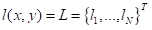
       训练过程中，使用BCEWithLogitsLoss(二元交叉熵损失函数)作为损失函数。若要理解BCEWithLogitsLoss，则应先熟悉BCELoss，该损失函数用来创建目标和输出之间的二进制交叉熵标准，使用公式表达如下：

其中，和 分别为网络输出(output)和目标(target)， 为权重， 为尺寸大小(batchsize)。

       BCEWithLogitsLoss损失函数相当于在BCELoss损失函数的基础上增加了Sigmoid层，即将输入数据规范为0-1之间，其计算公式如下：

其中，表示Sigmoid激活函数。

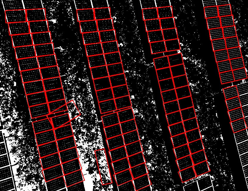
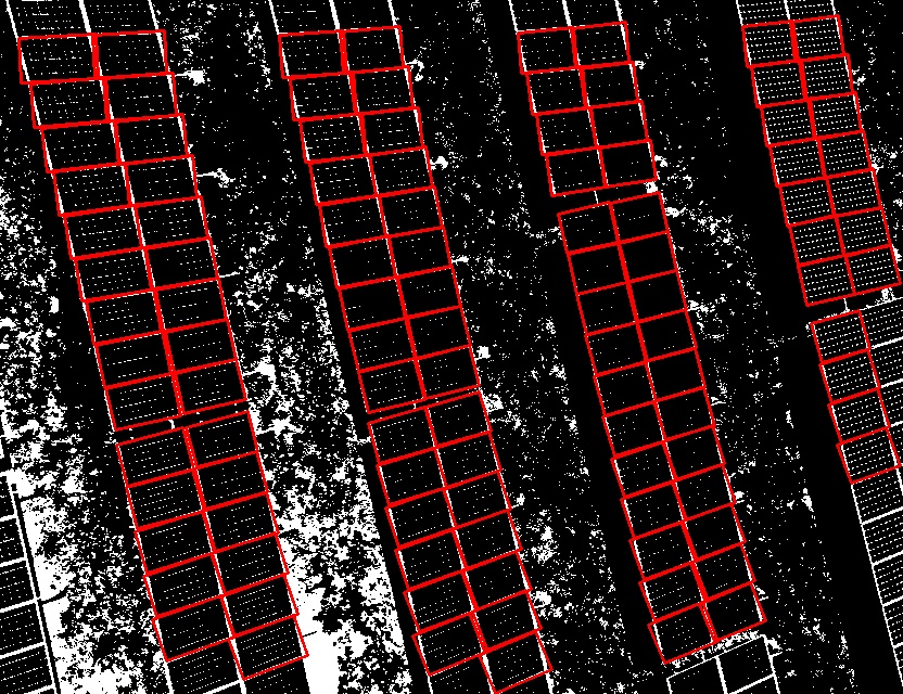
       本次实验中，对光伏电板图像中组件的边缘进行标记，大约标记了100张图片作为训练数据集。对该数据集进行训练，大约训练30轮左右，即可得到很好的测试效果。下面给出两组数据的测试结果：

                

        从这两组光伏电板图片的边缘分割测试结果来看，每一个组件的边缘均可以被清晰地分割出来，而没有组件遗漏和边缘误判的情况。而如果不使用深度学习的图像分割算法，采用之前介绍的例如阈值分割的传统图像处理方法对图像中的组件进行分割，则会造成因大量噪声而导致误判的情况。在此仅仅介绍了U-Net一种属于深度学习的图像分割算法，如有机会，可自行研究和尝试DeepLab系列等语义分割算法，或可得到很好的分割效果。