梯度下降法:
【转载时请注明来源】:http://www.cnblogs.com/runner-ljt/
Ljt
作为一个初学者,水平有限,欢迎交流指正。
应用:求线性回归方程的系数
目标:最小化损失函数 (损失函数定义为残差的平方和)
搜索方向:负梯度方向,负梯度方向是下降最快的方向
梯度下降法的R实现
#Gradient Descent 梯度下降法
# 在直接设置固定的step时,不宜设置的过大,当步长过大时会报错:
# Error in while ((newerror > error) | (iter < maxiter)) { :  missing value where TRUE/FALSE needed
#原因是step过大,会导致在迭代过程中梯度会特别的大,当超过1e+309时就会直接变成无穷Inf

#梯度下降法求线性回归方程系数theta
#x为数据矩阵(mxn m:样本数 n:特征数 );y观测值(mx1);error终止条件,相邻两次搜索结果的幅度;
#step为设定的固定步长;maxiter最大迭代次数,alpha,beta为回溯下降法的参数
GradientDescent<-function(x,y,error,maxiter,stepmethod=T,step=0.001,alpha=0.25,beta=0.8)
{
  m<-nrow(x)
  x<-cbind(matrix(1,m,1),x)
  n<-ncol(x)
  theta<-matrix(rep(0,n),n,1)  #theta初始值都设置为0
  iter<-1
  newerror<-1

while((newerror>error)|(iter<maxiter)){
    iter<-iter+1
    h<-x%*%theta
    des<-t(t(h-y)%*%x)  #梯度
#回溯下降法求步长t
       if(stepmethod==T){
            sstep=1
            new_theta<-theta-sstep*des
            new_h<-x%*%new_theta
            costfunction<-t(h-y)%*%(h-y)  #最小二乘损失函数
            new_costfunction<-t(new_h-y)%*%(new_h-y)
            #回溯下降法求步长sstep
            while(new_costfunction>costfunction-alpha*sstep*sum(des*des)){
                  sstep<-sstep*beta
                  new_theta<-theta-sstep*des
                  new_h<-x%*%new_theta
                  new_costfunction<-t(new_h-y)%*%(new_h-y)
                 }
            newerror<-t(theta-new_theta)%*%(theta-new_theta)
            theta<-new_theta
         }

#直接设置固定步长
      if(stepmethod==F){
          new_theta<-theta-step*des
          new_h<-x%*%new_theta
         # new_costfunction<-t(new_h-y)%*%(new_h-y)
          newerror<-t(theta-new_theta)%*%(theta-new_theta)
          theta<-new_theta
       }

 }
      costfunction<-t(x%*%theta-y)%*%(x%*%theta-y)
      result<-list(theta,iter,costfunction)
      names(result)<-c('系数','迭代次数','误差')
      result
}
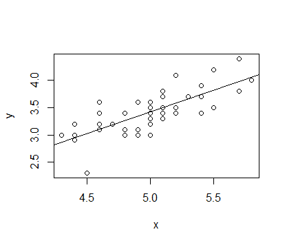
选取 IRIS 数据中种类为setosa的Sepal.Length和Sepal.Width数据分别作为x,y进行拟合,拟合函数为 y=α+βx
结果如下
> x<-matrix(iris[1:50,1],50,1)
> y<-matrix(iris[1:50,2],50,1)
> l<-lm(y~x)
> summary(l)

Call:
lm(formula = y ~ x)

Residuals:
     Min       1Q   Median       3Q      Max
-0.72394 -0.18273 -0.00306  0.15738  0.51709

Coefficients:
            Estimate Std. Error t value Pr(>|t|)
(Intercept)  -0.5694     0.5217  -1.091    0.281
x             0.7985     0.1040   7.681 6.71e-10 ***
---
Signif. codes:  0 ‘***’ 0.001 ‘**’ 0.01 ‘*’ 0.05 ‘.’ 0.1 ‘ ’ 1

Residual standard error: 0.2565 on 48 degrees of freedom
Multiple R-squared:  0.5514,	Adjusted R-squared:  0.542
F-statistic: 58.99 on 1 and 48 DF,  p-value: 6.71e-10

>
> GradientDescent(x,y,1e-14,1000,stepmethod=T,step=0.001,alpha=0.25,beta=0.8)
$系数
           [,1]
[1,] -0.5692863
[2,]  0.7984992

$迭代次数
[1] 23785

$误差
         [,1]
[1,] 3.158675

>
> GradientDescent(x,y,1e-14,1000,stepmethod=F,step=0.001,alpha=0.25,beta=0.8)
$系数
           [,1]
[1,] -0.5690111
[2,]  0.7984445

$迭代次数
[1] 31882

$误差
         [,1]
[1,] 3.158675