感谢中国人民大学胡鹤老师,课讲得非常好~
首先,何谓tensor?即高维向量,例如矩阵是二维,tensor是更广义意义上的n维向量(有type+shape)
TensorFlow执行过程为定义图,其中定义子节点,计算时只计算所需节点所依赖的节点,是一种高效且适应大规模的数据计算,方便分布式设计,对于复杂神经网络的计算,可将其拆开到其他核中同时计算。
Theano——torch———caffe(尤其是图像处理)——deeplearning5j——H20——MXNet,TensorFlow
运行环境
下载docker
打开docker quickstart terminal
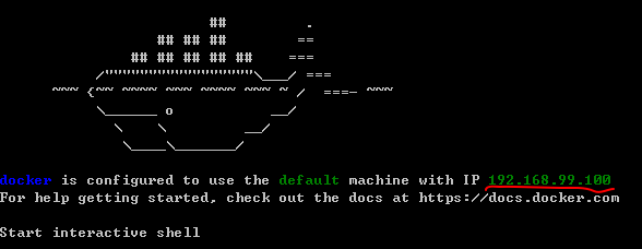
标红地方显示该docker虚拟机IP地址(即之后的localhost)
docker tensorflow/tensorflow //自动找到TensorFlow容器并下载
docker images //浏览当前容器
docker run -p 8888:8888 tensorflow/tensorflow //在8888端口运行
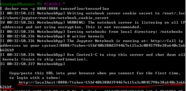
会出现一个token,复制该链接并替换掉localhost,既可以打开TensorFlow的一个编写器,jupyter
大体雏形
#python导入
import tensorflow as tf
#定义变量(节点)
x = tf.Variable(3, name="x")
y = tf.Variable(4, name="y")
f = x*x*y + y + 2
#定义session
sess = tf.Session()
#为已经定义的节点赋值
sess.run(x.initializer)
sess.run(y.initializer)
#运行session
result = sess.run(f)
print(result)  #42
#释放空间
sess.close
还有一个更简洁的一种定义并运行session方法
# a better way
with tf.Session() as sess:
    x.initializer.run()
    y.initializer.run()
    #即evaluate,求解f的值
    result = f.eval()
初始化的两行也可以写作
init = tf.global_variables_initializer()
init.run()
而session可以改作sess=tf.InteractiveSession()运行起来更方便
init = tf.global_variables_initializer()
sess = tf.InteractiveSession()
init.run()
result = f.eval()
print(result)
因而TensorFlow的代码分为两部分,定义部分和执行部分
TensorFlow是一个图的操作,有自动缺省的默认图和你自己定义的图
#系统默认缺省的图
>>> x1 = tf.Variable(1)
>>> x1.graph is tf.get_default_graph()
True
#自定义的图
>>> graph = tf.Graph()
>>> with graph.as_default():
x2 = tf.Variable(2)
>>> x2.graph is graph
True
>>> x2.graph is tf.get_default_graph()
False
节点的生命周期
第二种方法可以找出公共部分,避免x被计算2次。
运行结束后所有节点的值都被清空,如果没有单独保存,还需重新run一遍。
w = tf.constant(3)
x = w + 2
y = x + 5
z = x * 3
with tf.Session() as sess:
    print(y.eval()) # 10
    print(z.eval()) # 15

with tf.Session() as sess:
    y_val, z_val = sess.run([y, z])
    print(y_val) # 10
    print(z_val) # 15
Linear Regression with TensorFlow(线性回归上的应用)
y = wx+b = wx' //这里x'是相较于x多了一维全是1的向量
这里引用California housing的数据
TensorFlow上向量是列向量,需要reshape(-1,1)即转置成列向量
使用normal equation方法求解
import numpy as np
from sklearn.datasets import fetch_california_housing
housing = fetch_california_housing()
#获得数据维度,矩阵的行列长度
m, n = housing.data.shape
#np.c_是连接的含义,加了一个全为1的维度
housing_data_plus_bias = np.c_[np.ones((m, 1)), housing.data]
#数据量并不大,可以直接用常量节点装载进来,但是之后海量数据无法使用(会用minbatch的方式导入数据)
X = tf.constant(housing_data_plus_bias, dtype=tf.float32, name="X")
#转置成列向量
y = tf.constant(housing.target.reshape(-1, 1), dtype=tf.float32, name="y")
XT = tf.transpose(X)
#使用normal equation的方法求解theta,之前线性模型中有提及
theta = tf.matmul(tf.matmul(tf.matrix_inverse(tf.matmul(XT, X)), XT), y)
#求出权重
with tf.Session() as sess:
    theta_value = theta.eval()
如果是原本的方法,可能更直接些。但由于使用底层的库不同,它们计算出来的值不完全相同。
#使用numpy
X = housing_data_plus_bias
y = housing.target.reshape(-1, 1)
theta_numpy = np.linalg.inv(X.T.dot(X)).dot(X.T).dot(y)
#使用sklearn
from sklearn.linear_model import LinearRegression
lin_reg = LinearRegression()
lin_reg.fit(housing.data, housing.target.reshape(-1, 1))
这里不禁感到疑惑,为什么TensorFlow感觉变复杂了呢?其实,这不过因为这里数据规模较小,进行大规模的计算时,TensorFlow的自动优化所发挥的效果,是十分厉害的。
使用gradient descent(梯度下降)方法求解
#使用gradient时需要scale一下
from sklearn.preprocessing import StandardScaler
scaler = StandardScaler()
scaled_housing_data = scaler.fit_transform(housing.data)
scaled_housing_data_plus_bias = np.c_[np.ones((m, 1)), scaled_housing_data]
#迭代1000次
n_epochs = 1000
learning_rate = 0.01
#由于使用gradient,写入x的值需要scale一下
X = tf.constant(scaled_housing_data_plus_bias, dtype=tf.float32, name="X")
y = tf.constant(housing.target.reshape(-1, 1), dtype=tf.float32, name="y")
#使用gradient需要有一个初值
theta = tf.Variable(tf.random_uniform([n + 1, 1], -1.0, 1.0), name="theta")
#当前预测的y,x是m*(n+1),theta是(n+1)*1,刚好是y的维度
y_pred = tf.matmul(X, theta, name="predictions")
#整体误差
error = y_pred - y
#TensorFlow求解均值功能强大,可以指定维数,也可以像下面方法求整体的
mse = tf.reduce_mean(tf.square(error), name="mse")
#暂时自己写出训练过程,实际可以采用TensorFlow自带的功能更强大的自动求解autodiff方法
gradients = 2/m * tf.matmul(tf.transpose(X), error)
training_op = tf.assign(theta, theta - learning_rate * gradients)
#初始化并开始求解
init = tf.global_variables_initializer()
with tf.Session() as sess:
    sess.run(init)
    for epoch in range(n_epochs):
        #每运行100次打印一下当前平均误差
        if epoch % 100 == 0:
            print("Epoch", epoch, "MSE =", mse.eval())
        sess.run(training_op)
    best_theta = theta.eval()
上述代码中的autodiff如下,可以自动求出gradient
gradients = tf.gradients(mse, [theta])[0]
使用Optimizer
上述的整个梯度下降和迭代方法,都封装了在如下方法中
optimizer = tf.train.GradientDescentOptimizer(learning_rate=learning_rate)
training_op = optimizer.minimize(mse)
这样的optimizer还有很多
例如带冲量的optimizer = tf.train.MomentumOptimizer(learning_rate=learning_rate,momentum=0.9)
Feeding data to training algorithm
当数据量达到几G,几十G时,使用constant直接导入数据显然是不现实的,因而我们用placeholder做一个占位符
(一般行都是none,即数据量是任意的)
真正运行,run的时候再feed数据。可以不断使用新的数据。
>>> A = tf.placeholder(tf.float32, shape=(None, 3))
>>> B = A + 5
>>> with tf.Session() as sess:
... B_val_1 = B.eval(feed_dict={A: [[1, 2, 3]]})
... B_val_2 = B.eval(feed_dict={A: [[4, 5, 6], [7, 8, 9]]})
...
>>> print(B_val_1)
[[ 6. 7. 8.]]
>>> print(B_val_2)
[[ 9. 10. 11.]
[ 12. 13. 14.]]
这样,就可以通过定义min_batch来分批次随机抽取指定数量的数据,即便是几T的数据也可以抽取。
batch_size = 100
n_batches = int(np.ceil(m / batch_size))
#有放回的随机抽取数据
def fetch_batch(epoch, batch_index, batch_size):
    #定义一个随机种子
    np.random.seed(epoch * n_batches + batch_index)  # not shown in the book
    indices = np.random.randint(m, size=batch_size)  # not shown
    X_batch = scaled_housing_data_plus_bias[indices] # not shown
    y_batch = housing.target.reshape(-1, 1)[indices] # not shown
    return X_batch, y_batch
#开始运行
with tf.Session() as sess:
    sess.run(init)
#每次都抽取新的数据做训练
    for epoch in range(n_epochs):
        for batch_index in range(n_batches):
            X_batch, y_batch = fetch_batch(epoch, batch_index, batch_size)
            sess.run(training_op, feed_dict={X: X_batch, y: y_batch})
#最终结果
    best_theta = theta.eval()
Saving and Restoring models(保存模型)
有时候,运行几天的模型可能因故暂时无法继续跑下去,因而需要暂时保持已训练好的部分模型到硬盘上。
init = tf.global_variables_initializer()
saver = tf.train.Saver()
#保存模型
with tf.Session() as sess:
    sess.run(init)

    for epoch in range(n_epochs):
        if epoch % 100 == 0:
            #print("Epoch", epoch, "MSE =", mse.eval())
            save_path = saver.save(sess, "/tmp/my_model.ckpt")
        sess.run(training_op)

    best_theta = theta.eval()
    save_path = saver.save(sess, "/tmp/my_model_final.ckpt")
#恢复模型
with tf.Session() as sess:
    saver.restore(sess, "/tmp/my_model_final.ckpt")
    best_theta_restored = theta.eval()
关于TensorBoard
众所周知,神经网络和机器学习大多是黑盒模型,让人有点忐忑。TensorBoard所起的功能就是将这个黑盒稍微变白一些~
启用tensorboard
输入docker ps查看当前容器id
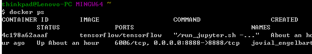
进入容器

使用tensorboard --log-dir=tf_logs命令打开已经存入的tf_logs文件,其生成代码如下所示
from datetime import datetime

now = datetime.utcnow().strftime("%Y%m%d%H%M%S")
root_logdir = "tf_logs"
logdir = "{}/run-{}/".format(root_logdir, now)
...
mse_summary = tf.summary.scalar('MSE', mse)
file_writer = tf.summary.FileWriter(logdir, tf.get_default_graph())
...
if batch_index % 10 == 0:
                summary_str = mse_summary.eval(feed_dict={X: X_batch, y: y_batch})
                step = epoch * n_batches + batch_index
                file_writer.add_summary(summary_str, step)