最近几个月一直在和几个小伙伴做Deep Learning相关的事情。除了像tensorflow,gpu这些框架或工具之外,最大的收获是思路上的,Neural Network相当富余变化,发挥所想、根据手头的数据和问题去设计创新吧。今天聊一个Unsupervised Learning的NN:Autoencoder。
Autoencoder的特点是:首先,数据中只有X,没有y;此外,输入和输出的nodes数量相同,可以把其定义为用神经网络对input data压缩、取精华后的重构。其结构图如下:
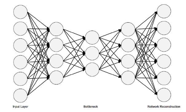
听起来蛮抽象,但从其architecture上面,来看,首先是全连接(fully-connected network)。和Feed-forward NN的重点不同是,FFNN的neurons per layer逐层递减,而Autoencoder则是neurons per layer先减少,这部分叫做Encode,中间存在一个瓶颈层,然后再逐渐放大至原先的size,这部分叫做Decode。然后在output layer,希望输出和输入一致,以此思路构建loss function (MSE),然后再做Back-propagation。
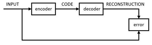
工作流图如下:
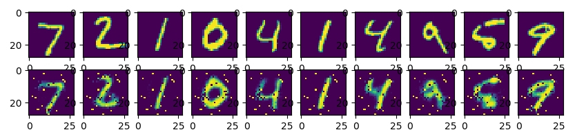
数据集用的是MNIST手写数字库,encode有3层,decode有3层,核心代码可见最下方。压缩并还原之后,得出的图片对比如下,可见Autoencoder虽然在bottleneck处将数据压缩了很多,但经过decode之后,基本是可以还原图片数据的 :
当然,如果压缩再解压,得到差不多的图片,其实意义不大,那我们考虑在训练结束后,只用encode的部分,即Autoencoder的前半部来给数据做降维,那么会得到什么结果呢?在这个例子中,为了更好地把数据降到2维,我加了另外2层hidden layer,并且bottleneck层移除了activation function,得到的结果如下:
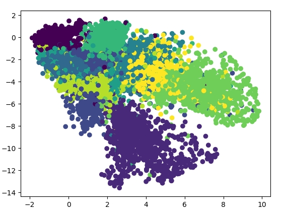
可以看到,数据被从784维空间中压缩到2维,并且做了类似clustering的操作。
# Parameter
learning_rate = 0.001
training_epochs = 50
batch_size = 256
display_step = 1
examples_to_show = 10

# Network Parameters
n_input = 784  # MNIST data input (img shape: 28*28)

# hidden layer settings
n_hidden_1 = 256 # 1st layer num features
n_hidden_2 = 128 # 2nd layer num features
n_hidden_3 = 64  # 3rd layer num features

X = tf.placeholder(tf.float32, [None,n_input])

weights = {
    'encoder_h1':tf.Variable(tf.random_normal([n_input,n_hidden_1])),
    'encoder_h2': tf.Variable(tf.random_normal([n_hidden_1,n_hidden_2])),
    'encoder_h3': tf.Variable(tf.random_normal([n_hidden_2,n_hidden_3])),
    'decoder_h1': tf.Variable(tf.random_normal([n_hidden_3,n_hidden_2])),
    'decoder_h2': tf.Variable(tf.random_normal([n_hidden_2,n_hidden_1])),
    'decoder_h3': tf.Variable(tf.random_normal([n_hidden_1, n_input])),
    }
biases = {
    'encoder_b1': tf.Variable(tf.random_normal([n_hidden_1])),
    'encoder_b2': tf.Variable(tf.random_normal([n_hidden_2])),
    'encoder_b3': tf.Variable(tf.random_normal([n_hidden_3])),
    'decoder_b1': tf.Variable(tf.random_normal([n_hidden_2])),
    'decoder_b2': tf.Variable(tf.random_normal([n_hidden_1])),
    'decoder_b3': tf.Variable(tf.random_normal([n_input])),
    }

# Building the encoder
def encoder(x):
    # Encoder Hidden layer with sigmoid activation #1
    layer_1 = tf.nn.sigmoid(tf.add(tf.matmul(x, weights['encoder_h1']),
                                   biases['encoder_b1']))
    # Decoder Hidden layer with sigmoid activation #2
    layer_2 = tf.nn.sigmoid(tf.add(tf.matmul(layer_1, weights['encoder_h2']),
                                   biases['encoder_b2']))
    layer_3 = tf.nn.sigmoid(tf.add(tf.matmul(layer_2, weights['encoder_h3']),
                                   biases['encoder_b3']))
    return layer_3

# Building the decoder
def decoder(x):
    # Encoder Hidden layer with sigmoid activation #1
    layer_1 = tf.nn.sigmoid(tf.add(tf.matmul(x, weights['decoder_h1']),
                                   biases['decoder_b1']))
    # Decoder Hidden layer with sigmoid activation #2
    layer_2 = tf.nn.sigmoid(tf.add(tf.matmul(layer_1, weights['decoder_h2']),
                                   biases['decoder_b2']))
    layer_3 = tf.nn.sigmoid(tf.add(tf.matmul(layer_2, weights['decoder_h3']),
                                   biases['decoder_b3']))
    return layer_3

# Construct model
encoder_op = encoder(X)             # 128 Features
decoder_op = decoder(encoder_op)    # 784 Features

# Prediction
y_pred = decoder_op    # After
# Targets (Labels) are the input data.
y_true = X            # Before

# Define loss and optimizer, minimize the squared error
cost = tf.reduce_mean(tf.pow(y_true - y_pred, 2))
optimizer = tf.train.AdamOptimizer(learning_rate).minimize(cost)

# Launch the graph
with tf.Session() as sess:
    sess.run(tf.global_variables_initializer())
    total_batch = int(mnist.train.num_examples/batch_size)
    # Training cycle
    for epoch in range(training_epochs):
        # Loop over all batches
        for i in range(total_batch):
            batch_xs, batch_ys = mnist.train.next_batch(batch_size)  # max(x) = 1, min(x) = 0
            # Run optimization op (backprop) and cost op (to get loss value)
            _, c = sess.run([optimizer, cost], feed_dict={X: batch_xs})
        # Display logs per epoch step
        if epoch % display_step == 0:
            print("Epoch:", '%04d' % (epoch+1),
                  "cost=", "{:.9f}".format(c))

    print("Optimization Finished!")