k近邻学习的一种实现时k-d树,用于搜索一个给定的向量周围k个与他距离最近的向量,好像ACM的数据结构里面也有着一条。
基于线性扫描算法的k近邻学习算法适合于处理数据集比较小的情况,时间复杂度大约是O(nlogn),搜索到这k个最近的向量之后就可以根据他们的众数选择属于哪一个类比较适合
k-d树代码:
import numpy as np
from queue import deque
import heapq

class KDTree:
    def __init__(self, k_neighbors=5):
        # 保存最近邻居数k
        self.k_neighbors = k_neighbors

    def _node_depth(self, i):
        '''计算节点深度'''

        t = np.log2(i + 2)
        return int(t) + (0 if t.is_integer() else 1)

    def _kd_tree_build(self, X):
        '''构造KD-Tree'''

        m, n = X.shape
        tree_depth = self._node_depth(m - 1)
        M = 2 ** tree_depth - 1

        # 节点由两个索引构成:
        # [0]实例索引, [1]切分特征索引.
        tree = np.zeros((M, 2), dtype=np.int)
        tree[:, 0] = -1

        # 利用队列层序创建KD-Tree.
        indices = np.arange(m)
        queue = deque([[0, 0, indices]])
        while queue:
            # 队列中弹出一项包括:
            # 树节点索引, 切分特征索引, 当前区域所有实例索引.
            i, l, indices = queue.popleft()
            # 以实例第l个特征中位数作为切分点进行切分
            k = indices.size // 2
            indices = indices[np.argpartition(X[indices, l], k)]
            # 保存切分点实例到当前节节点
            tree[i, 0] = indices[k]
            tree[i, 1] = l

            # 循环使用下一特征作为切分特征
            l = (l + 1) % n
            # 将切分点左右区域的节点划分到左右子树: 将实例索引入队, 创建左右子树.
            li, ri = 2 * i + 1, 2 * i + 2
            if indices.size > 1:
                queue.append([li, l, indices[:k]])
            if indices.size > 2:
                queue.append([ri, l, indices[k+1:]])

        # 返回树及树的深度
        return tree, tree_depth

    def _kd_tree_search(self, x, root, X, res_heap):
        '''搜索KD-Tree, 将最近的k个邻居放入大端堆.'''

        i = root
        idx = self.tree[i, 0]
        # 判断节点是否存在, 若不存在则返回.
        if idx < 0:
            return

        # 获取当前root节点深度
        depth = self._node_depth(i)
        # 移动到x所在最小超矩形区域相应的叶节点
        for _ in range(self.tree_depth - depth):
            s = X[idx]
            # 获取当前节点切分特征索引
            l = self.tree[i, 1]
            # 根据当前节点切分特征的值, 选择移动到左儿子或右儿子节点.
            if x[l] <= s[l]:
                i = i * 2 + 1
            else:
                i = i * 2 + 2
            idx = self.tree[i, 0]

        if idx > 0:
            # 计算到叶节点中实例的距离
            s = X[idx]
            d = np.linalg.norm(x - s)

            # 进行入堆出堆操作, 更新当前k个最近邻居和最近距离.
            heapq.heappushpop(res_heap, (-d, idx))

        while i > root:
            # 计算到父节点中实例的距离, 并更新当前最近距离.
            parent_i = (i - 1) // 2
            parent_idx = self.tree[parent_i, 0]
            parent_s = X[parent_idx]
            d = np.linalg.norm(x - parent_s)

            # 进行入堆出堆操作, 更新当前k个最近邻居和最近距离.
            heapq.heappushpop(res_heap, (-d, parent_idx))

            # 获取切分特征索引
            l = self.tree[parent_i, 1]
            # 获取超球体半径
            r = -res_heap[0][0]
            # 判断超球体(x, r)是否与兄弟节点区域相交
            if np.abs(x[l] - parent_s[l]) < r:
                # 获取兄弟节点的树索引
                sibling_i = (i + 1) if i % 2 else (i - 1)
                # 递归搜索兄弟子树
                self._kd_tree_search(x, sibling_i, X, res_heap)

            # 递归向根节点回退
            i = parent_i

    def train(self, X_train, y_train):
        '''训练'''

        # 保存训练集
        self.X_train = X_train
        self.y_train = y_train

        # 构造k-d树, 保存树及树的深度.
        self.tree, self.tree_depth = self._kd_tree_build(X_train)

    def _predict_one(self, x):
        '''对单个实例进行预测'''

        # 创建存储k个最近邻居索引的最大堆.
        # 注意: 标准库中的heapq实现的是最小堆, 以距离的负数作为键则等价与最大堆.
        res_heap = [(-np.inf, -1)] * self.k_neighbors
        # 从根开始搜索kd tree, 将最近的k个邻居将存入堆.
        self._kd_tree_search(x, 0, self.X_train, res_heap)
        # 获取k个邻居的索引
        indices = [idx for _, idx in res_heap]

        # 投票法:
        # 1.统计k个邻居中各类别出现的个数
        counts = np.bincount(self.y_train[indices])
        # 2.返回最频繁出现的类别
        return np.argmax(counts)

    def predict(self, X):
        '''预测'''

        # 对X中每个实例依次调用_predict_one方法进行预测.
        return np.apply_along_axis(self._predict_one, 1, X)
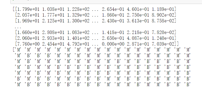
使用乳腺癌的样本进行分类
http://archive.ics.uci.edu/ml/machine-learning-databases/breast-cancer-wisconsin/
import numpy as np
X=np.genfromtxt('F:/python_test/data/wdbc.data',delimiter=',',usecols=range(2,32))
print(X)
y=np.genfromtxt('F:/python_test/data/wdbc.data',delimiter=',',usecols=1,dtype=np.str)
print(y)
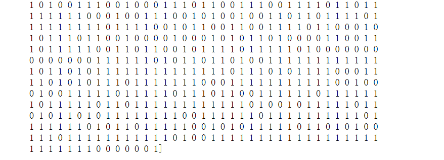
y=np.where(y == 'B',1,0)
print(y)
选择周围的三个样本训练和拟合,准确度还比较高的,计算了在k=3的情况下的单次准确度以及平均准确度
clf=KDTree(3)
from sklearn.model_selection import train_test_split
X_train,X_test,y_train,y_test = train_test_split(X,y,test_size=0.3)
clf.train(X_train,y_train)
from sklearn.metrics import accuracy_score
y_pred=clf.predict(X_test)
accuracy=accuracy_score(y_test,y_pred)
print(accuracy)

def test(X,y,k):
    X_train,X_test,y_train,y_test = train_test_split(X,y,test_size=0.3)
    clf=KDTree(k)
    clf.train(X_train,y_train)
    y_pred=clf.predict(X_test)
    accuracy=accuracy_score(y_test,y_pred)

    return accuracy

accuracy_mean=np.mean([test(X,y,3) for _ in range(50)])
得到平均的准确度是0.9243274853801169
下面将数据进行最大最小值标准化,将原来的属性中的每一个值都映射到[0,1]区间中去,
from sklearn.preprocessing import MinMaxScaler
def test(X,y,k):
    X_train,X_test,y_train,y_test = train_test_split(X,y,test_size=0.3)

    mms = MinMaxScaler()
    X_train_norm = mms.fit_transform(X_train)
    X_test_norm = mms.transform(X_test)

    clf=KDTree(k)
    clf.train(X_train_norm,y_train)
    y_pred=clf.predict(X_test_norm)
    accuracy=accuracy_score(y_test,y_pred)

    return accuracy

accuracy_mean=np.mean([test(X,y,3) for _ in range(50)])

下面通过搜索确定最佳的k值,一般k值是取奇数,这样的话保证了两个类别数量一定可以比较出大小
K = list(range(1,20,2))
print(K)
acc_array=[[test(X,y,k) for _ in range(50)] for k in K]
print(acc_array)

计算平均精确度
np.mean(acc_array,axis=1)

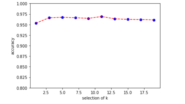
绘制变化图像,发现k的选择并没有对结果有太大的影响
import matplotlib.pyplot as plt
K = list(range(1,20,2))
plt.scatter(K,mean_arr,color='blue')
plt.plot(K,mean_arr,color='red',linestyle='--')
plt.xlabel('selection of k')
plt.ylabel('accuracy')
plt.ylim([0.8,1.0])
plt.show()