灰度直方图
介绍
实现
以下代码便于理解灰度直方图的计算,其中histogram函数是基于numpy简化的,运行结果如下。
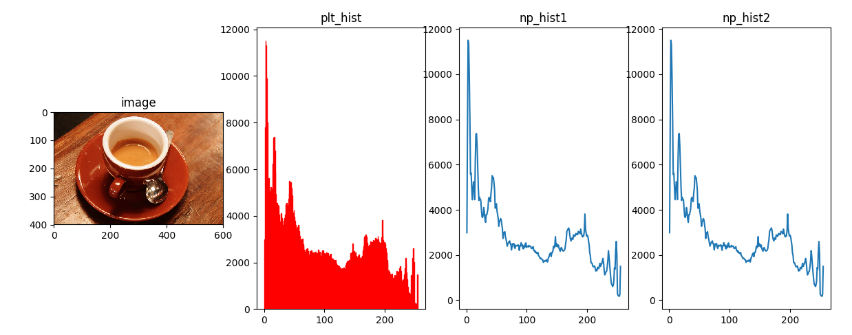
# coding: utf8
from skimage import data
import matplotlib.pyplot as plt
import numpy as np

def histogram(a, bins=10, range=None):
    """
    Compute the histogram of a set of data.

    """
    import numpy as np
    from numpy.core import linspace
    from numpy.core.numeric import (arange, asarray)
    # 转成一维数组
    a = asarray(a)
    a = a.ravel()
    mn, mx = [mi + 0.0 for mi in range]
    ntype = np.dtype(np.intp)
    n = np.zeros(bins, ntype)
    # 预计算直方图缩放因子
    norm = bins / (mx - mn)

    # 均分,计算边缘以进行潜在的校正
    bin_edges = linspace(mn, mx, bins + 1, endpoint=True)

    # 分块对于大数组可以降低运行内存,同时提高速度
    BLOCK = 65536
    for i in arange(0, len(a), BLOCK):
        tmp_a = a[i:i + BLOCK]
        tmp_a_data = tmp_a.astype(float)
        # 减去Range下限,乘以缩放因子,向下取整
        tmp_a = tmp_a_data - mn
        tmp_a *= norm
        indices = tmp_a.astype(np.intp)
        # 对indices标签分别计数,标签等于bins减一
        indices[indices == bins] -= 1
        n += np.bincount(indices, weights=None,
                             minlength=bins).astype(ntype)

    return n, bin_edges

if __name__ =="__main__":
    img=data.coffee()

    fig = plt.figure()
    f1 = fig.add_subplot(141)
    f1.imshow(img)
    f1.set_title("image")

    f2 = fig.add_subplot(142)
    arr=img.flatten()
    n, bins, patches = f2.hist(arr, bins=256, facecolor='red')
    f2.set_title("plt_hist")

    f3 = fig.add_subplot(143)
    hist, others = np.histogram(arr, range=(0, arr.max()), bins=256)
    f3.plot(others[1:],hist)
    f3.set_title("np_hist1")

    f4 = fig.add_subplot(144)
    hist, others = histogram(arr, range=(0, arr.max()), bins=256)
    f4.plot(others[1:], hist)
    f4.set_title("np_hist2")
    plt.show()
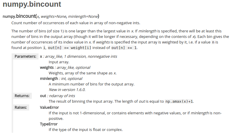
关于bincount函数,可以参考Xurtle的博文https://blog.csdn.net/xlinsist/article/details/51346523
bin的数量比x中的最大值大1,每个bin给出了它的索引值在x中出现的次数。下面,我举个例子让大家更好的理解一下:
# 我们可以看到x中最大的数为7,因此bin的数量为8,那么它的索引值为0->7
x = np.array([0, 1, 1, 3, 2, 1, 7])
# 索引0出现了1次,索引1出现了3次......索引5出现了0次......
np.bincount(x)
#因此,输出结果为:array([1, 3, 1, 1, 0, 0, 0, 1])

# 我们可以看到x中最大的数为7,因此bin的数量为8,那么它的索引值为0->7
x = np.array([7, 6, 2, 1, 4])
# 索引0出现了0次,索引1出现了1次......索引5出现了0次......
np.bincount(x)
#输出结果为:array([0, 1, 1, 0, 1, 0, 1, 1])
下面,我来解释一下weights这个参数。文档说,如果weights参数被指定,那么x会被它加权,也就是说,如果值n发现在位置i,那么out[n] += weight[i]而不是out[n] += 1.因此,我们weights的大小必须与x相同,否则报错。下面,我举个例子让大家更好的理解一下:
w = np.array([0.3, 0.5, 0.2, 0.7, 1., -0.6])
# 我们可以看到x中最大的数为4,因此bin的数量为5,那么它的索引值为0->4
x = np.array([2, 1, 3, 4, 4, 3])
# 索引0 -> 0
# 索引1 -> w[1] = 0.5
# 索引2 -> w[0] = 0.3
# 索引3 -> w[2] + w[5] = 0.2 - 0.6 = -0.4
# 索引4 -> w[3] + w[4] = 0.7 + 1 = 1.7
np.bincount(x, weights=w)
# 因此,输出结果为:array([ 0. , 0.5, 0.3, -0.4, 1.7])
最后,我们来看一下minlength这个参数。文档说,如果minlength被指定,那么输出数组中bin的数量至少为它指定的数(如果必要的话,bin的数量会更大,这取决于x)。下面,我举个例子让大家更好的理解一下:
# 我们可以看到x中最大的数为3,因此bin的数量为4,那么它的索引值为0->3
x = np.array([3, 2, 1, 3, 1])
# 本来bin的数量为4,现在我们指定了参数为7,因此现在bin的数量为7,所以现在它的索引值为0->6
np.bincount(x, minlength=7)
# 因此,输出结果为:array([0, 2, 1, 2, 0, 0, 0])

# 我们可以看到x中最大的数为3,因此bin的数量为4,那么它的索引值为0->3
x = np.array([3, 2, 1, 3, 1])
# 本来bin的数量为4,现在我们指定了参数为1,那么它指定的数量小于原本的数量,因此这个参数失去了作用,索引值还是0->3
np.bincount(x, minlength=1)
# 因此,输出结果为:array([0, 2, 1, 2])
直方图均衡化
直方图均衡化是一种通过使用图像直方图,调整对比度的图像处理方法;通过对图像的强度(intensity)进行某种非线性变换,使得变换后的图像直方图为近似均匀分布,从而,达到提高图像对比度和增强图片的目的。普通的直方图均衡化采用如下形式的非线性变换:
设 f 为原始灰度图像,g 为直方图均衡化的灰度图像,则 g 和 f 的每个像素的映射关系如下:
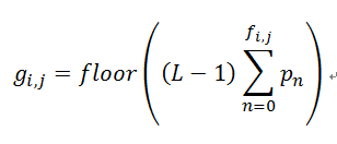
其中,L 为灰度级,通常为 256,表明了图像像素的强度的范围为 0 ~ L-1;
pn 等于图像 f 中强度为 n 的像素数占总像素数的比例,即原始灰度图直方图的概率密度函数;
fi,j 表示在图像 f 中,第 i 行,第 j 列的像素强度;gi,j 表示在图像 g 中,第 i 行,第 j 列的像素强度.
Python代码
实现如下,代码和图片转自https://www.cnblogs.com/klchang/p/9872363.html
运行结果为
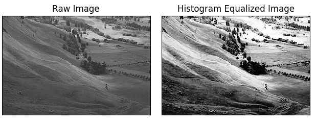
从输出看,将原来0-255的灰度范围差异放大,起到了增强对比的效果。
#!/usr/bin/env python
# -*- coding: utf8 -*-
"""
# Author: klchang
# Date: 2018.10
# Description:
    histogram equalization of a gray image.
"""
from __future__ import print_function
import numpy as np
import matplotlib.pyplot as plt


def histequ(gray, nlevels=256):
    # Compute histogram
    histogram = np.bincount(gray.flatten(), minlength=nlevels)
    print ("histogram: ", histogram)

    # Mapping function
    uniform_hist = (nlevels - 1) * (np.cumsum(histogram)/(gray.size * 1.0))
    uniform_hist = uniform_hist.astype('uint8')
    print ("uniform hist: ", uniform_hist)

    # Set the intensity of the pixel in the raw gray to its corresponding new intensity
    height, width = gray.shape
    uniform_gray = np.zeros(gray.shape, dtype='uint8')  # Note the type of elements
    for i in range(height):
        for j in range(width):
            uniform_gray[i,j] = uniform_hist[gray[i,j]]

    return uniform_gray


if __name__ == '__main__':
    fname = "../320px-Unequalized_Hawkes_Bay_NZ.png" # Gray image
    # Note, matplotlib natively only read png images.
    gray = plt.imread(fname, format=np.uint8)
    if gray is None:
        print ("Image {} does not exist!".format(fname))
        exit(-1)

    # Histogram equalization
    uniform_gray = histequ(gray)

    # Display the result
    fig, (ax1, ax2) = plt.subplots(1, 2)
    ax1.set_title("Raw Image")
    ax1.imshow(gray, 'gray')
    ax1.set_xticks([]), ax1.set_yticks([])

    ax2.set_title("Histogram Equalized Image")
    ax2.imshow(uniform_gray, 'gray')
    ax2.set_xticks([]), ax2.set_yticks([])

    fig.tight_layout()
    plt.show()
"""
histogram:  [   0    0    0    0    0    0    0    0    0    0    0    0    0    0    0
    0    0    0    0    0    0    0    0    0    0    0    0    0    0    0
    0    0    0    0    0    0    0    0    0    0    0    0    0    0    0
    0    0    0    0    0    0    0    0    0    0    0    0    0    0    0
    0    0    0    0    0    0    0    0    0    0    0    0    0    0    0
    0    0    0    0    0    0    0    0    0    0    0    0    0    0    0
    0    0    0    0    0    0    0    0    0    1    0    0    0    1    0
    0    1    1    1    2    2    2    6    9   10   17   33   34   35   55
   69   95  122  188  206  249  312  349  485  644  798 1042 1285 1536 1807
 2241 2542 2921 2862 2586 2398 2259 2092 1897 1986 1860 1724 1782 1673 1772
 1632 1670 1716 1595 1478 1466 1271 1197 1066 1028  908  827  807  764  671
  606  547  461  417  414  379  347  273  290  273  207  226  198  184  158
  171  149  122  133  144  126  137  135  121  118  133  137  158  153  147
  138  161  126  128   97   96   46   47   41   37   26   14   10    7   12
    6    2    5    3    1    1    0    1    0    0    0    0    1    0    1
    0    0    1    0    0    0    0    0    0    0    0    0    0    0    0
    0    0    0    0    0    0    0    0    0    0    0    0    0    0    0
    0]
uniform hist:  [  0   0   0   0   0   0   0   0   0   0   0   0   0   0   0   0   0   0
   0   0   0   0   0   0   0   0   0   0   0   0   0   0   0   0   0   0
   0   0   0   0   0   0   0   0   0   0   0   0   0   0   0   0   0   0
   0   0   0   0   0   0   0   0   0   0   0   0   0   0   0   0   0   0
   0   0   0   0   0   0   0   0   0   0   0   0   0   0   0   0   0   0
   0   0   0   0   0   0   0   0   0   0   0   0   0   0   0   0   0   0
   0   0   0   0   0   0   0   0   0   0   0   0   1   1   1   2   3   4
   5   6   8  10  13  17  22  28  35  43  53  63  74  84  93 101 109 116
 124 131 137 144 150 157 163 169 175 181 187 192 197 202 206 209 213 216
 219 222 224 227 229 230 232 233 235 236 237 238 239 240 241 242 242 243
 244 244 245 245 246 246 247 247 248 248 249 249 250 250 251 251 252 252
 253 253 254 254 254 254 254 254 254 254 254 254 254 254 254 254 254 254
 254 254 254 254 254 254 254 254 254 254 254 255 255 255 255 255 255 255
 255 255 255 255 255 255 255 255 255 255 255 255 255 255 255 255 255 255
 255 255 255 255]
"""