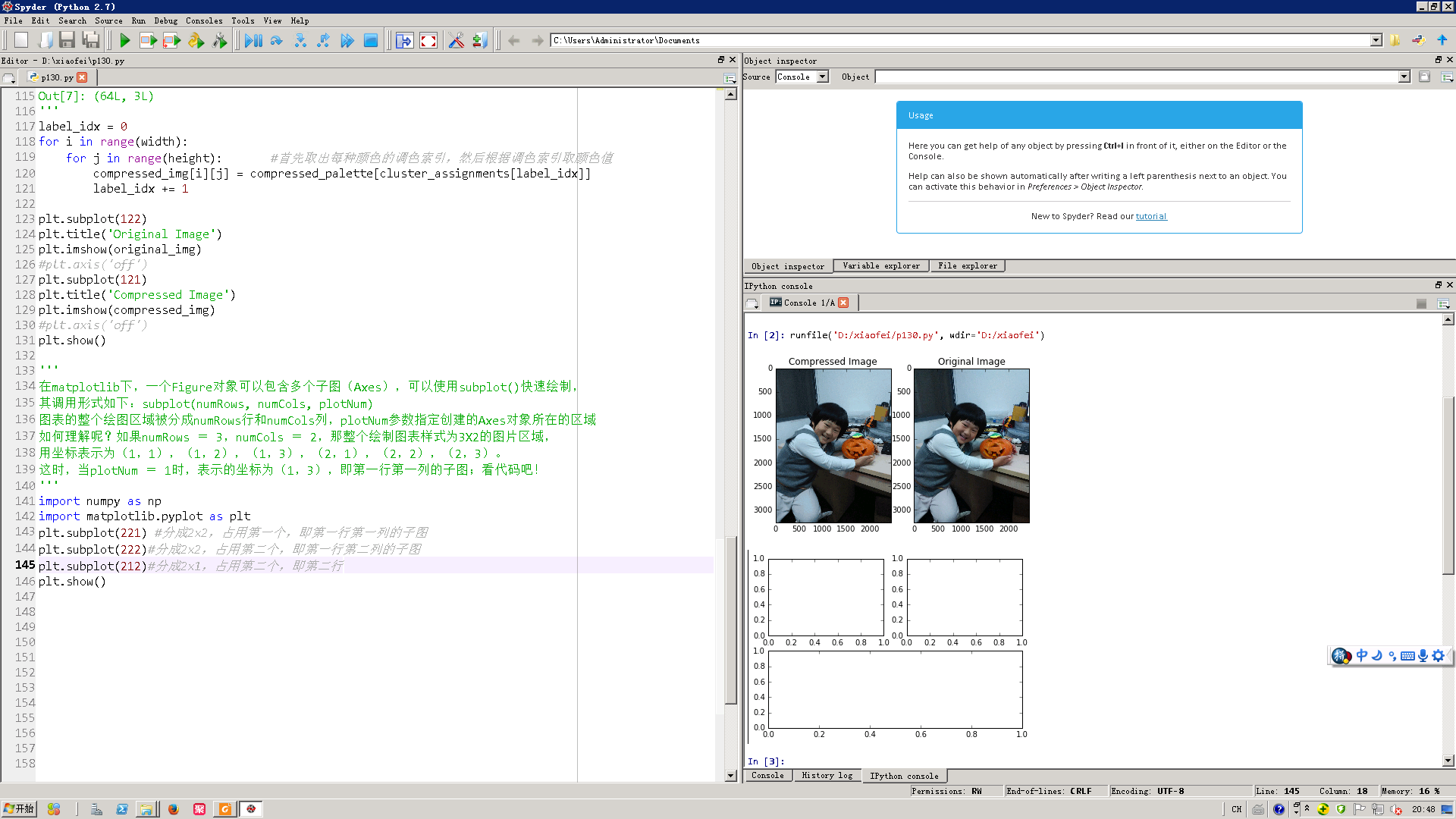
# -*- coding: utf-8 -*-
"""
Created on Thu Aug 11 18:54:12 2016

@author: Administrator
"""

import numpy as np
import  matplotlib.pyplot as plt
from sklearn.cluster import KMeans
from sklearn.utils import shuffle
import mahotas as mh

original_img = np.array(mh.imread('haonan.jpg'), dtype=np.float64) / 255
original_dimensions = tuple(original_img.shape)
width, height, depth = tuple(original_img.shape)
#(3264L, 2448L, 3L)
image_flattened = np.reshape(original_img, (width * height, depth))
#(7990272L, 3L)
#将原始的图像,变成多行的样式

#打乱图像像素,选取1000个
image_array_sample = shuffle(image_flattened,random_state=0)[:1000]

#聚集为64个颜色
estimator = KMeans(n_clusters=64, random_state=0)
estimator.fit(image_array_sample)


#Next, we predict the cluster assignment for each of the pixels in the original image:
#将7990272L颜色划分为64种
cluster_assignments = estimator.predict(image_flattened)
'''
cluster_assignments.shape
Out[19]: (7990272L,)
'''
#Finally, we create the compressed image from the compressed palette and cluster assignments:

compressed_palette = estimator.cluster_centers_
'''
compressed_palette.shape
Out[3]: (64L, 3L)

compressed_palette
Out[4]:
array([[ 0.54188948,  0.66987522,  0.73404635],
       [ 0.16122004,  0.20232389,  0.22962963],
       [ 0.06970588,  0.06088235,  0.06794118],
       [ 0.34392157,  0.46039216,  0.53215686],
       [ 0.68235294,  0.29254902,  0.04862745],
       [ 0.2619281 ,  0.34901961,  0.41911765],
       [ 0.68074866,  0.80784314,  0.86737968],
       [ 0.54313725,  0.57843137,  0.57647059],
       [ 0.47882353,  0.36588235,  0.32117647],
       [ 0.11993464,  0.15108932,  0.17821351],
       [ 0.7745098 ,  0.4745098 ,  0.31372549],
       [ 0.62459893,  0.73698752,  0.7983066 ],
       [ 0.81764706,  0.95098039,  0.57843137],
       [ 0.0248366 ,  0.01837755,  0.02568243],
       [ 0.28912656,  0.22816399,  0.20071301],
       [ 0.44456328,  0.44955437,  0.42245989],
       [ 0.19869281,  0.27215686,  0.33856209],
       [ 0.14588235,  0.12797386,  0.12130719],
       [ 0.51568627,  0.21372549,  0.04019608],
       [ 0.68333333,  0.59411765,  0.53431373],
       [ 0.43227753,  0.5040724 ,  0.56440422],
       [ 0.37167756,  0.29803922,  0.26143791],
       [ 0.73908497,  0.86248366,  0.91477124],
       [ 0.55882353,  0.64215686,  0.7004902 ],
       [ 0.70812325,  0.72941176,  0.71820728],
       [ 0.75215686,  0.37098039,  0.11372549],
       [ 0.20980392,  0.72156863,  0.59411765],
       [ 0.57896613,  0.69875223,  0.75995247],
       [ 0.40588235,  0.08529412,  0.01372549],
       [ 0.55764706,  0.45490196,  0.20470588],
       [ 0.41921569,  0.56352941,  0.65411765],
       [ 0.29877451,  0.4129902 ,  0.4877451 ],
       [ 0.08686275,  0.12215686,  0.16686275],
       [ 0.30532213,  0.32156863,  0.34117647],
       [ 0.51980392,  0.61686275,  0.66823529],
       [ 0.51078431,  0.51666667,  0.50686275],
       [ 0.16642157,  0.24730392,  0.30514706],
       [ 0.0629156 ,  0.07212276,  0.09445865],
       [ 0.6373366 ,  0.75955882,  0.82295752],
       [ 0.13777778,  0.17934641,  0.20836601],
       [ 0.65098039,  0.65588235,  0.66176471],
       [ 0.49338235,  0.57867647,  0.63578431],
       [ 0.33823529,  0.37205882,  0.37745098],
       [ 0.2047619 ,  0.30532213,  0.38207283],
       [ 0.20980392,  0.04313725,  0.02941176],
       [ 0.19758673,  0.2361991 ,  0.26033183],
       [ 0.59215686,  0.26143791,  0.01699346],
       [ 0.24145658,  0.17086835,  0.13893557],
       [ 0.50532213,  0.49971989,  0.43417367],
       [ 0.79215686,  0.45196078,  0.21372549],
       [ 0.12529412,  0.20078431,  0.26431373],
       [ 0.59691028,  0.71895425,  0.78193702],
       [ 0.51764706,  0.2745098 ,  0.17647059],
       [ 0.62058824,  0.51911765,  0.46911765],
       [ 0.60952381,  0.68095238,  0.73977591],
       [ 0.11687812,  0.0946559 ,  0.09265667],
       [ 0.28627451,  0.25359477,  0.25294118],
       [ 0.08411765,  0.09392157,  0.11764706],
       [ 0.74845938,  0.76246499,  0.77983193],
       [ 0.62287582,  0.26339869,  0.09607843],
       [ 0.84313725,  0.94901961,  0.42745098],
       [ 0.43267974,  0.41045752,  0.36601307],
       [ 0.65918833,  0.77756498,  0.84012768],
       [ 0.04037763,  0.03384168,  0.04139434]])
'''
#生成一个新的图像,全部是0,深度和原来图像相等
compressed_img = np.zeros((width, height, compressed_palette.shape[1]))
'''
compressed_palette.shape
Out[7]: (64L, 3L)
'''
label_idx = 0
for i in range(width):
    for j in range(height):       #首先取出每种颜色的调色索引,然后根据调色索引取颜色值
        compressed_img[i][j] = compressed_palette[cluster_assignments[label_idx]]
        label_idx += 1

plt.subplot(122)
plt.title('Original Image')
plt.imshow(original_img)
#plt.axis('off')
plt.subplot(121)
plt.title('Compressed Image')
plt.imshow(compressed_img)
#plt.axis('off')
plt.show()

'''
在matplotlib下,一个Figure对象可以包含多个子图(Axes),可以使用subplot()快速绘制,
其调用形式如下:subplot(numRows, numCols, plotNum)
图表的整个绘图区域被分成numRows行和numCols列,plotNum参数指定创建的Axes对象所在的区域
如何理解呢?如果numRows = 3,numCols = 2,那整个绘制图表样式为3X2的图片区域,
用坐标表示为(1,1),(1,2),(1,3),(2,1),(2,2),(2,3)。
这时,当plotNum = 1时,表示的坐标为(1,3),即第一行第一列的子图;看代码吧!
'''
import numpy as np
import matplotlib.pyplot as plt
plt.subplot(221) #分成2x2,占用第一个,即第一行第一列的子图
plt.subplot(222)#分成2x2,占用第二个,即第一行第二列的子图
plt.subplot(212)#分成2x1,占用第二个,即第二行
plt.show()