Statistical functions
#Percent change
Series and DataFrame have a method pct_change() (opens new window)to compute the percent change over a given number of periods (using fill_method to fill NA/null values before computing the percent change).
In [1]: ser = pd.Series(np.random.randn(8))

In [2]: ser.pct_change()
Out[2]:
0         NaN
1   -1.602976
2    4.334938
3   -0.247456
4   -2.067345
5   -1.142903
6   -1.688214
7   -9.759729
dtype: float64

In [3]: df = pd.DataFrame(np.random.randn(10, 4))

In [4]: df.pct_change(periods=3)
Out[4]:
          0         1         2         3
0       NaN       NaN       NaN       NaN
1       NaN       NaN       NaN       NaN
2       NaN       NaN       NaN       NaN
3 -0.218320 -1.054001  1.987147 -0.510183
4 -0.439121 -1.816454  0.649715 -4.822809
5 -0.127833 -3.042065 -5.866604 -1.776977
6 -2.596833 -1.959538 -2.111697 -3.798900
7 -0.117826 -2.169058  0.036094 -0.067696
8  2.492606 -1.357320 -1.205802 -1.558697
9 -1.012977  2.324558 -1.003744 -0.371806
Covariance
Series.cov() (opens new window)can be used to compute covariance between series (excluding missing values).
In [5]: s1 = pd.Series(np.random.randn(1000))

In [6]: s2 = pd.Series(np.random.randn(1000))

In [7]: s1.cov(s2)
Out[7]: 0.000680108817431082
Analogously, DataFrame.cov() (opens new window)to compute pairwise covariances among the series in the DataFrame, also excluding NA/null values.
Note
Assuming the missing data are missing at random this results in an estimate for the covariance matrix which is unbiased. However, for many applications this estimate may not be acceptable because the estimated covariance matrix is not guaranteed to be positive semi-definite. This could lead to estimated correlations having absolute values which are greater than one, and/or a non-invertible covariance matrix. See Estimation of covariance matrices (opens new window)for more details.
In [8]: frame = pd.DataFrame(np.random.randn(1000, 5),
   ...:                      columns=['a', 'b', 'c', 'd', 'e'])
   ...:

In [9]: frame.cov()
Out[9]:
          a         b         c         d         e
a  1.000882 -0.003177 -0.002698 -0.006889  0.031912
b -0.003177  1.024721  0.000191  0.009212  0.000857
c -0.002698  0.000191  0.950735 -0.031743 -0.005087
d -0.006889  0.009212 -0.031743  1.002983 -0.047952
e  0.031912  0.000857 -0.005087 -0.047952  1.042487
DataFrame.cov also supports an optional min_periods keyword that specifies the required minimum number of observations for each column pair in order to have a valid result.
In [10]: frame = pd.DataFrame(np.random.randn(20, 3), columns=['a', 'b', 'c'])

In [11]: frame.loc[frame.index[:5], 'a'] = np.nan

In [12]: frame.loc[frame.index[5:10], 'b'] = np.nan

In [13]: frame.cov()
Out[13]:
          a         b         c
a  1.123670 -0.412851  0.018169
b -0.412851  1.154141  0.305260
c  0.018169  0.305260  1.301149

In [14]: frame.cov(min_periods=12)
Out[14]:
          a         b         c
a  1.123670       NaN  0.018169
b       NaN  1.154141  0.305260
c  0.018169  0.305260  1.301149
Correlation
Correlation may be computed using the corr() (opens new window)method. Using the method parameter, several methods for computing correlations are provided:
| Method name | Description |
|---|---|
| pearson (default) | Standard correlation coefficient |
| kendall | Kendall Tau correlation coefficient |
| spearman | Spearman rank correlation coefficient |
All of these are currently computed using pairwise complete observations. Wikipedia has articles covering the above correlation coefficients:
- Pearson correlation coefficient(opens new window)
- Kendall rank correlation coefficient(opens new window)
- Spearman’s rank correlation coefficient(opens new window)
Note
Please see the caveats associated with this method of calculating correlation matrices in the covariance section.
In [15]: frame = pd.DataFrame(np.random.randn(1000, 5),
   ....:                      columns=['a', 'b', 'c', 'd', 'e'])
   ....:

In [16]: frame.iloc[::2] = np.nan

# Series with Series
In [17]: frame['a'].corr(frame['b'])
Out[17]: 0.013479040400098794

In [18]: frame['a'].corr(frame['b'], method='spearman')
Out[18]: -0.007289885159540637

# Pairwise correlation of DataFrame columns
In [19]: frame.corr()
Out[19]:
          a         b         c         d         e
a  1.000000  0.013479 -0.049269 -0.042239 -0.028525
b  0.013479  1.000000 -0.020433 -0.011139  0.005654
c -0.049269 -0.020433  1.000000  0.018587 -0.054269
d -0.042239 -0.011139  0.018587  1.000000 -0.017060
e -0.028525  0.005654 -0.054269 -0.017060  1.000000
Note that non-numeric columns will be automatically excluded from the correlation calculation.
Like cov, corr also supports the optional min_periods keyword:
In [20]: frame = pd.DataFrame(np.random.randn(20, 3), columns=['a', 'b', 'c'])

In [21]: frame.loc[frame.index[:5], 'a'] = np.nan

In [22]: frame.loc[frame.index[5:10], 'b'] = np.nan

In [23]: frame.corr()
Out[23]:
          a         b         c
a  1.000000 -0.121111  0.069544
b -0.121111  1.000000  0.051742
c  0.069544  0.051742  1.000000

In [24]: frame.corr(min_periods=12)
Out[24]:
          a         b         c
a  1.000000       NaN  0.069544
b       NaN  1.000000  0.051742
c  0.069544  0.051742  1.000000
The method argument can also be a callable for a generic correlation calculation. In this case, it should be a single function that produces a single value from two ndarray inputs. Suppose we wanted to compute the correlation based on histogram intersection:
# histogram intersection
In [25]: def histogram_intersection(a, b):
   ....:     return np.minimum(np.true_divide(a, a.sum()),
   ....:                       np.true_divide(b, b.sum())).sum()
   ....:

In [26]: frame.corr(method=histogram_intersection)
Out[26]:
          a          b          c
a  1.000000  -6.404882  -2.058431
b -6.404882   1.000000 -19.255743
c -2.058431 -19.255743   1.000000
A related method corrwith() (opens new window)is implemented on DataFrame to compute the correlation between like-labeled Series contained in different DataFrame objects.
In [27]: index = ['a', 'b', 'c', 'd', 'e']

In [28]: columns = ['one', 'two', 'three', 'four']

In [29]: df1 = pd.DataFrame(np.random.randn(5, 4), index=index, columns=columns)

In [30]: df2 = pd.DataFrame(np.random.randn(4, 4), index=index[:4], columns=columns)

In [31]: df1.corrwith(df2)
Out[31]:
one     -0.125501
two     -0.493244
three    0.344056
four     0.004183
dtype: float64

In [32]: df2.corrwith(df1, axis=1)
Out[32]:
a   -0.675817
b    0.458296
c    0.190809
d   -0.186275
e         NaN
dtype: float64
Data ranking
The rank() (opens new window)method produces a data ranking with ties being assigned the mean of the ranks (by default) for the group:
In [33]: s = pd.Series(np.random.np.random.randn(5), index=list('abcde'))

In [34]: s['d'] = s['b']  # so there's a tie

In [35]: s.rank()
Out[35]:
a    5.0
b    2.5
c    1.0
d    2.5
e    4.0
dtype: float64
rank() (opens new window)is also a DataFrame method and can rank either the rows (axis=0) or the columns (axis=1). NaN values are excluded from the ranking.
In [36]: df = pd.DataFrame(np.random.np.random.randn(10, 6))

In [37]: df[4] = df[2][:5]  # some ties

In [38]: df
Out[38]:
          0         1         2         3         4         5
0 -0.904948 -1.163537 -1.457187  0.135463 -1.457187  0.294650
1 -0.976288 -0.244652 -0.748406 -0.999601 -0.748406 -0.800809
2  0.401965  1.460840  1.256057  1.308127  1.256057  0.876004
3  0.205954  0.369552 -0.669304  0.038378 -0.669304  1.140296
4 -0.477586 -0.730705 -1.129149 -0.601463 -1.129149 -0.211196
5 -1.092970 -0.689246  0.908114  0.204848       NaN  0.463347
6  0.376892  0.959292  0.095572 -0.593740       NaN -0.069180
7 -1.002601  1.957794 -0.120708  0.094214       NaN -1.467422
8 -0.547231  0.664402 -0.519424 -0.073254       NaN -1.263544
9 -0.250277 -0.237428 -1.056443  0.419477       NaN  1.375064

In [39]: df.rank(1)
Out[39]:
     0    1    2    3    4    5
0  4.0  3.0  1.5  5.0  1.5  6.0
1  2.0  6.0  4.5  1.0  4.5  3.0
2  1.0  6.0  3.5  5.0  3.5  2.0
3  4.0  5.0  1.5  3.0  1.5  6.0
4  5.0  3.0  1.5  4.0  1.5  6.0
5  1.0  2.0  5.0  3.0  NaN  4.0
6  4.0  5.0  3.0  1.0  NaN  2.0
7  2.0  5.0  3.0  4.0  NaN  1.0
8  2.0  5.0  3.0  4.0  NaN  1.0
9  2.0  3.0  1.0  4.0  NaN  5.0
rank optionally takes a parameter ascending which by default is true; when false, data is reverse-ranked, with larger values assigned a smaller rank.
rank supports different tie-breaking methods, specified with the method parameter:
average: average rank of tied groupmin: lowest rank in the groupmax: highest rank in the groupfirst: ranks assigned in the order they appear in the array
#Window Functions
For working with data, a number of window functions are provided for computing common window or rolling statistics. Among these are count, sum, mean, median, correlation, variance, covariance, standard deviation, skewness, and kurtosis.
The rolling() and expanding() functions can be used directly from DataFrameGroupBy objects, see the groupby docs.
Note
The API for window statistics is quite similar to the way one works with GroupBy objects, see the documentation here.
We work with rolling, expanding and exponentially weighted data through the corresponding objects, Rolling, Expanding and EWM.
In [40]: s = pd.Series(np.random.randn(1000),
   ....:               index=pd.date_range('1/1/2000', periods=1000))
   ....:

In [41]: s = s.cumsum()

In [42]: s
Out[42]:
2000-01-01    -0.268824
2000-01-02    -1.771855
2000-01-03    -0.818003
2000-01-04    -0.659244
2000-01-05    -1.942133
                ...
2002-09-22   -67.457323
2002-09-23   -69.253182
2002-09-24   -70.296818
2002-09-25   -70.844674
2002-09-26   -72.475016
Freq: D, Length: 1000, dtype: float64
These are created from methods on Series and DataFrame.
In [43]: r = s.rolling(window=60)

In [44]: r
Out[44]: Rolling [window=60,center=False,axis=0]
These object provide tab-completion of the available methods and properties.
In [14]: r.<TAB>                                          # noqa: E225, E999
r.agg         r.apply       r.count       r.exclusions  r.max         r.median      r.name        r.skew        r.sum
r.aggregate   r.corr        r.cov         r.kurt        r.mean        r.min         r.quantile    r.std         r.var
Generally these methods all have the same interface. They all accept the following arguments:
window: size of moving windowmin_periods: threshold of non-null data points to require (otherwise result is NA)center: boolean, whether to set the labels at the center (default is False)
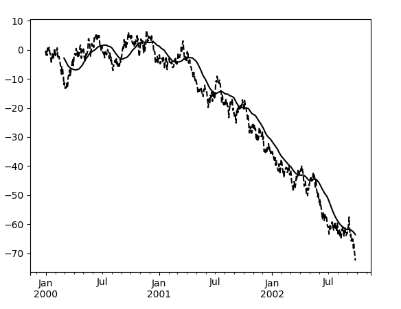
We can then call methods on these rolling objects. These return like-indexed objects:
In [45]: r.mean()
Out[45]:
2000-01-01          NaN
2000-01-02          NaN
2000-01-03          NaN
2000-01-04          NaN
2000-01-05          NaN
                ...
2002-09-22   -62.914971
2002-09-23   -63.061867
2002-09-24   -63.213876
2002-09-25   -63.375074
2002-09-26   -63.539734
Freq: D, Length: 1000, dtype: float64
In [46]: s.plot(style='k--')
Out[46]: <matplotlib.axes._subplots.AxesSubplot at 0x7f66048bdef0>

In [47]: r.mean().plot(style='k')
Out[47]: <matplotlib.axes._subplots.AxesSubplot at 0x7f66048bdef0>
They can also be applied to DataFrame objects. This is really just syntactic sugar for applying the moving window operator to all of the DataFrame’s columns:
In [48]: df = pd.DataFrame(np.random.randn(1000, 4),
   ....:                   index=pd.date_range('1/1/2000', periods=1000),
   ....:                   columns=['A', 'B', 'C', 'D'])
   ....:

In [49]: df = df.cumsum()

In [50]: df.rolling(window=60).sum().plot(subplots=True)
Out[50]:
array([<matplotlib.axes._subplots.AxesSubplot object at 0x7f66075a7f60>,
       <matplotlib.axes._subplots.AxesSubplot object at 0x7f65f79e55c0>,
       <matplotlib.axes._subplots.AxesSubplot object at 0x7f65f7998588>,
       <matplotlib.axes._subplots.AxesSubplot object at 0x7f65f794b550>],
      dtype=object)

Method summary
We provide a number of common statistical functions:
| Method | Description |
|---|---|
| count() |
Number of non-null observations |
| sum() |
Sum of values |
| mean() |
Mean of values |
| median() |
Arithmetic median of values |
| min() |
Minimum |
| max() |
Maximum |
| std() |
Bessel-corrected sample standard deviation |
| var() |
Unbiased variance |
| skew() |
Sample skewness (3rd moment) |
| kurt() |
Sample kurtosis (4th moment) |
| quantile() |
Sample quantile (value at %) |
| apply() |
Generic apply |
| cov() |
Unbiased covariance (binary) |
| corr() |
Correlation (binary) |
The apply() (opens new window)function takes an extra func argument and performs generic rolling computations. The func argument should be a single function that produces a single value from an ndarray input. Suppose we wanted to compute the mean absolute deviation on a rolling basis:
In [51]: def mad(x):
   ....:     return np.fabs(x - x.mean()).mean()
   ....:

In [52]: s.rolling(window=60).apply(mad, raw=True).plot(style='k')
Out[52]: <matplotlib.axes._subplots.AxesSubplot at 0x7f65f795fac8>

Rolling windows
Passing win_type to .rolling generates a generic rolling window computation, that is weighted according the win_type. The following methods are available:
| Method | Description |
|---|---|
| sum() |
Sum of values |
| mean() |
Mean of values |
The weights used in the window are specified by the win_type keyword. The list of recognized types are the scipy.signal window functions (opens new window):
boxcartriangblackmanhammingbartlettparzenbohmanblackmanharrisnuttallbarthannkaiser(needs beta)gaussian(needs std)general_gaussian(needs power, width)slepian(needs width)exponential(needs tau).
In [53]: ser = pd.Series(np.random.randn(10),
   ....:                 index=pd.date_range('1/1/2000', periods=10))
   ....:

In [54]: ser.rolling(window=5, win_type='triang').mean()
Out[54]:
2000-01-01         NaN
2000-01-02         NaN
2000-01-03         NaN
2000-01-04         NaN
2000-01-05   -1.037870
2000-01-06   -0.767705
2000-01-07   -0.383197
2000-01-08   -0.395513
2000-01-09   -0.558440
2000-01-10   -0.672416
Freq: D, dtype: float64
Note that the boxcar window is equivalent to mean()
In [55]: ser.rolling(window=5, win_type='boxcar').mean()
Out[55]:
2000-01-01         NaN
2000-01-02         NaN
2000-01-03         NaN
2000-01-04         NaN
2000-01-05   -0.841164
2000-01-06   -0.779948
2000-01-07   -0.565487
2000-01-08   -0.502815
2000-01-09   -0.553755
2000-01-10   -0.472211
Freq: D, dtype: float64

In [56]: ser.rolling(window=5).mean()
Out[56]:
2000-01-01         NaN
2000-01-02         NaN
2000-01-03         NaN
2000-01-04         NaN
2000-01-05   -0.841164
2000-01-06   -0.779948
2000-01-07   -0.565487
2000-01-08   -0.502815
2000-01-09   -0.553755
2000-01-10   -0.472211
Freq: D, dtype: float64
For some windowing functions, additional parameters must be specified:
In [57]: ser.rolling(window=5, win_type='gaussian').mean(std=0.1)
Out[57]:
2000-01-01         NaN
2000-01-02         NaN
2000-01-03         NaN
2000-01-04         NaN
2000-01-05   -1.309989
2000-01-06   -1.153000
2000-01-07    0.606382
2000-01-08   -0.681101
2000-01-09   -0.289724
2000-01-10   -0.996632
Freq: D, dtype: float64
Note
For .sum() with a win_type, there is no normalization done to the weights for the window. Passing custom weights of [1, 1, 1] will yield a different result than passing weights of [2, 2, 2], for example. When passing a win_type instead of explicitly specifying the weights, the weights are already normalized so that the largest weight is 1.
In contrast, the nature of the .mean() calculation is such that the weights are normalized with respect to each other. Weights of [1, 1, 1] and [2, 2, 2] yield the same result.
Time-aware rolling
New in version 0.19.0.
New in version 0.19.0 are the ability to pass an offset (or convertible) to a .rolling() method and have it produce variable sized windows based on the passed time window. For each time point, this includes all preceding values occurring within the indicated time delta.
This can be particularly useful for a non-regular time frequency index.
In [58]: dft = pd.DataFrame({'B': [0, 1, 2, np.nan, 4]},
   ....:                    index=pd.date_range('20130101 09:00:00',
   ....:                                        periods=5,
   ....:                                        freq='s'))
   ....:

In [59]: dft
Out[59]:
                       B
2013-01-01 09:00:00  0.0
2013-01-01 09:00:01  1.0
2013-01-01 09:00:02  2.0
2013-01-01 09:00:03  NaN
2013-01-01 09:00:04  4.0
This is a regular frequency index. Using an integer window parameter works to roll along the window frequency.
In [60]: dft.rolling(2).sum()
Out[60]:
                       B
2013-01-01 09:00:00  NaN
2013-01-01 09:00:01  1.0
2013-01-01 09:00:02  3.0
2013-01-01 09:00:03  NaN
2013-01-01 09:00:04  NaN

In [61]: dft.rolling(2, min_periods=1).sum()
Out[61]:
                       B
2013-01-01 09:00:00  0.0
2013-01-01 09:00:01  1.0
2013-01-01 09:00:02  3.0
2013-01-01 09:00:03  2.0
2013-01-01 09:00:04  4.0
Specifying an offset allows a more intuitive specification of the rolling frequency.
In [62]: dft.rolling('2s').sum()
Out[62]:
                       B
2013-01-01 09:00:00  0.0
2013-01-01 09:00:01  1.0
2013-01-01 09:00:02  3.0
2013-01-01 09:00:03  2.0
2013-01-01 09:00:04  4.0
Using a non-regular, but still monotonic index, rolling with an integer window does not impart any special calculation.
In [63]: dft = pd.DataFrame({'B': [0, 1, 2, np.nan, 4]},
   ....:                    index=pd.Index([pd.Timestamp('20130101 09:00:00'),
   ....:                                    pd.Timestamp('20130101 09:00:02'),
   ....:                                    pd.Timestamp('20130101 09:00:03'),
   ....:                                    pd.Timestamp('20130101 09:00:05'),
   ....:                                    pd.Timestamp('20130101 09:00:06')],
   ....:                                   name='foo'))
   ....:

In [64]: dft
Out[64]:
                       B
foo
2013-01-01 09:00:00  0.0
2013-01-01 09:00:02  1.0
2013-01-01 09:00:03  2.0
2013-01-01 09:00:05  NaN
2013-01-01 09:00:06  4.0

In [65]: dft.rolling(2).sum()
Out[65]:
                       B
foo
2013-01-01 09:00:00  NaN
2013-01-01 09:00:02  1.0
2013-01-01 09:00:03  3.0
2013-01-01 09:00:05  NaN
2013-01-01 09:00:06  NaN
Using the time-specification generates variable windows for this sparse data.
In [66]: dft.rolling('2s').sum()
Out[66]:
                       B
foo
2013-01-01 09:00:00  0.0
2013-01-01 09:00:02  1.0
2013-01-01 09:00:03  3.0
2013-01-01 09:00:05  NaN
2013-01-01 09:00:06  4.0
Furthermore, we now allow an optional on parameter to specify a column (rather than the default of the index) in a DataFrame.
In [67]: dft = dft.reset_index()

In [68]: dft
Out[68]:
                  foo    B
0 2013-01-01 09:00:00  0.0
1 2013-01-01 09:00:02  1.0
2 2013-01-01 09:00:03  2.0
3 2013-01-01 09:00:05  NaN
4 2013-01-01 09:00:06  4.0

In [69]: dft.rolling('2s', on='foo').sum()
Out[69]:
                  foo    B
0 2013-01-01 09:00:00  0.0
1 2013-01-01 09:00:02  1.0
2 2013-01-01 09:00:03  3.0
3 2013-01-01 09:00:05  NaN
4 2013-01-01 09:00:06  4.0
Rolling window endpoints
New in version 0.20.0.
The inclusion of the interval endpoints in rolling window calculations can be specified with the closed parameter:
| closed | Description | Default for |
|---|---|---|
| right | close right endpoint | time-based windows |
| left | close left endpoint | |
| both | close both endpoints | fixed windows |
| neither | open endpoints |
For example, having the right endpoint open is useful in many problems that require that there is no contamination from present information back to past information. This allows the rolling window to compute statistics “up to that point in time”, but not including that point in time.
In [70]: df = pd.DataFrame({'x': 1},
   ....:                   index=[pd.Timestamp('20130101 09:00:01'),
   ....:                          pd.Timestamp('20130101 09:00:02'),
   ....:                          pd.Timestamp('20130101 09:00:03'),
   ....:                          pd.Timestamp('20130101 09:00:04'),
   ....:                          pd.Timestamp('20130101 09:00:06')])
   ....:

In [71]: df["right"] = df.rolling('2s', closed='right').x.sum()  # default

In [72]: df["both"] = df.rolling('2s', closed='both').x.sum()

In [73]: df["left"] = df.rolling('2s', closed='left').x.sum()

In [74]: df["neither"] = df.rolling('2s', closed='neither').x.sum()

In [75]: df
Out[75]:
                     x  right  both  left  neither
2013-01-01 09:00:01  1    1.0   1.0   NaN      NaN
2013-01-01 09:00:02  1    2.0   2.0   1.0      1.0
2013-01-01 09:00:03  1    2.0   3.0   2.0      1.0
2013-01-01 09:00:04  1    2.0   3.0   2.0      1.0
2013-01-01 09:00:06  1    1.0   2.0   1.0      NaN
Currently, this feature is only implemented for time-based windows. For fixed windows, the closed parameter cannot be set and the rolling window will always have both endpoints closed.
#Time-aware rolling vs. resampling
Using .rolling() with a time-based index is quite similar to resampling. They both operate and perform reductive operations on time-indexed pandas objects.
When using .rolling() with an offset. The offset is a time-delta. Take a backwards-in-time looking window, and aggregate all of the values in that window (including the end-point, but not the start-point). This is the new value at that point in the result. These are variable sized windows in time-space for each point of the input. You will get a same sized result as the input.
When using .resample() with an offset. Construct a new index that is the frequency of the offset. For each frequency bin, aggregate points from the input within a backwards-in-time looking window that fall in that bin. The result of this aggregation is the output for that frequency point. The windows are fixed size in the frequency space. Your result will have the shape of a regular frequency between the min and the max of the original input object.
To summarize, .rolling() is a time-based window operation, while .resample() is a frequency-based window operation.
#Centering windows
By default the labels are set to the right edge of the window, but a center keyword is available so the labels can be set at the center.
In [76]: ser.rolling(window=5).mean()
Out[76]:
2000-01-01         NaN
2000-01-02         NaN
2000-01-03         NaN
2000-01-04         NaN
2000-01-05   -0.841164
2000-01-06   -0.779948
2000-01-07   -0.565487
2000-01-08   -0.502815
2000-01-09   -0.553755
2000-01-10   -0.472211
Freq: D, dtype: float64

In [77]: ser.rolling(window=5, center=True).mean()
Out[77]:
2000-01-01         NaN
2000-01-02         NaN
2000-01-03   -0.841164
2000-01-04   -0.779948
2000-01-05   -0.565487
2000-01-06   -0.502815
2000-01-07   -0.553755
2000-01-08   -0.472211
2000-01-09         NaN
2000-01-10         NaN
Freq: D, dtype: float64
Binary window functions
cov() (opens new window)and corr() (opens new window)can compute moving window statistics about two Series or any combination of DataFrame/Series or DataFrame/DataFrame. Here is the behavior in each case:
- two
Series: compute the statistic for the pairing. DataFrame/Series: compute the statistics for each column of the DataFrame with the passed Series, thus returning a DataFrame.DataFrame/DataFrame: by default compute the statistic for matching column names, returning a DataFrame. If the keyword argumentpairwise=Trueis passed then computes the statistic for each pair of columns, returning aMultiIndexed DataFramewhoseindexare the dates in question (see the next section).
For example:
In [78]: df = pd.DataFrame(np.random.randn(1000, 4),
   ....:                   index=pd.date_range('1/1/2000', periods=1000),
   ....:                   columns=['A', 'B', 'C', 'D'])
   ....:

In [79]: df = df.cumsum()

In [80]: df2 = df[:20]

In [81]: df2.rolling(window=5).corr(df2['B'])
Out[81]:
                   A    B         C         D
2000-01-01       NaN  NaN       NaN       NaN
2000-01-02       NaN  NaN       NaN       NaN
2000-01-03       NaN  NaN       NaN       NaN
2000-01-04       NaN  NaN       NaN       NaN
2000-01-05  0.768775  1.0 -0.977990  0.800252
...              ...  ...       ...       ...
2000-01-16  0.691078  1.0  0.807450 -0.939302
2000-01-17  0.274506  1.0  0.582601 -0.902954
2000-01-18  0.330459  1.0  0.515707 -0.545268
2000-01-19  0.046756  1.0 -0.104334 -0.419799
2000-01-20 -0.328241  1.0 -0.650974 -0.777777

[20 rows x 4 columns]
Computing rolling pairwise covariances and correlations
In financial data analysis and other fields it’s common to compute covariance and correlation matrices for a collection of time series. Often one is also interested in moving-window covariance and correlation matrices. This can be done by passing the pairwise keyword argument, which in the case of DataFrame inputs will yield a MultiIndexed DataFrame whose index are the dates in question. In the case of a single DataFrame argument the pairwise argument can even be omitted:
Note
Missing values are ignored and each entry is computed using the pairwise complete observations. Please see the covariance section for caveats associated with this method of calculating covariance and correlation matrices.
In [82]: covs = (df[['B', 'C', 'D']].rolling(window=50)
   ....:                            .cov(df[['A', 'B', 'C']], pairwise=True))
   ....:

In [83]: covs.loc['2002-09-22':]
Out[83]:
                     B         C         D
2002-09-22 A  1.367467  8.676734 -8.047366
           B  3.067315  0.865946 -1.052533
           C  0.865946  7.739761 -4.943924
2002-09-23 A  0.910343  8.669065 -8.443062
           B  2.625456  0.565152 -0.907654
           C  0.565152  7.825521 -5.367526
2002-09-24 A  0.463332  8.514509 -8.776514
           B  2.306695  0.267746 -0.732186
           C  0.267746  7.771425 -5.696962
2002-09-25 A  0.467976  8.198236 -9.162599
           B  2.307129  0.267287 -0.754080
           C  0.267287  7.466559 -5.822650
2002-09-26 A  0.545781  7.899084 -9.326238
           B  2.311058  0.322295 -0.844451
           C  0.322295  7.038237 -5.684445
In [84]: correls = df.rolling(window=50).corr()

In [85]: correls.loc['2002-09-22':]
Out[85]:
                     A         B         C         D
2002-09-22 A  1.000000  0.186397  0.744551 -0.769767
           B  0.186397  1.000000  0.177725 -0.240802
           C  0.744551  0.177725  1.000000 -0.712051
           D -0.769767 -0.240802 -0.712051  1.000000
2002-09-23 A  1.000000  0.134723  0.743113 -0.758758
...                ...       ...       ...       ...
2002-09-25 D -0.739160 -0.164179 -0.704686  1.000000
2002-09-26 A  1.000000  0.087756  0.727792 -0.736562
           B  0.087756  1.000000  0.079913 -0.179477
           C  0.727792  0.079913  1.000000 -0.692303
           D -0.736562 -0.179477 -0.692303  1.000000

[20 rows x 4 columns]
You can efficiently retrieve the time series of correlations between two columns by reshaping and indexing:
In [86]: correls.unstack(1)[('A', 'C')].plot()
Out[86]: <matplotlib.axes._subplots.AxesSubplot at 0x7f65f8dc79e8>
