0 简介
0.1 主题

0.2 目标
0.2.1 能掌握聚类的距离计算方式
0.2.2 能够掌握聚类的各种方式
1 聚类定义

2 距离计算与相似度方法总结
2.1 距离算法


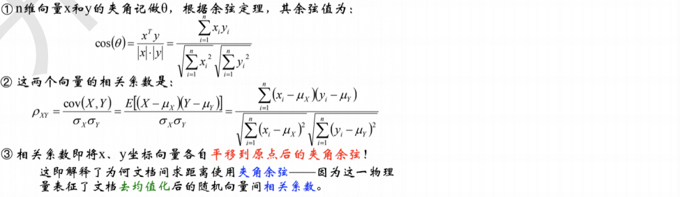
2.2 余弦相似度与Pearson相似度
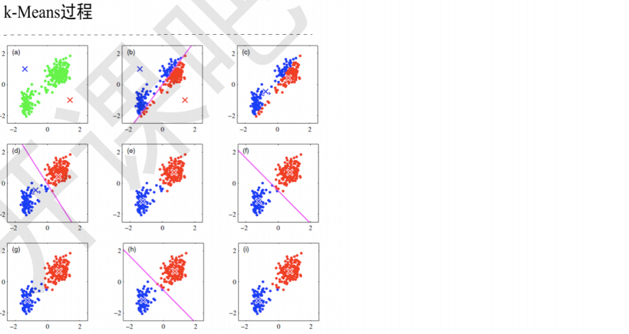
3 K-Means算法过程
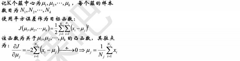
3.1 算法过程


3.2 代码实现
# 导入包
import numpy as np
import sklearn
from sklearn.datasets import make_blobs # 导入产生模拟数据的方法
from sklearn.cluster import KMeans # 导入kmeans 类
# 1. 产生模拟数据;random_state此参数让结果容易复现,随机过程跟系统时间有关
N = 100
centers = 4

X, Y = make_blobs(n_samples=N, n_features=2, centers=centers, random_state=28)
print(X)
# 2. 模型构建;init初始化函数的意思
km = KMeans(n_clusters=centers, init='random', random_state=28)
km.fit(X)
KMeans(algorithm='auto', copy_x=True, init='random', max_iter=300, n_clusters=4,
       n_init=10, n_jobs=None, precompute_distances='auto', random_state=28,
       tol=0.0001, verbose=0)
# 实际的y值
Y
array([0, 1, 3, 1, 2, 0, 3, 0, 0, 3, 0, 2, 1, 1, 3, 1, 0, 2, 0, 1, 0, 1,
       3, 1, 3, 0, 1, 3, 1, 1, 0, 0, 1, 3, 1, 0, 3, 2, 3, 1, 3, 3, 0, 2,
       2, 0, 2, 3, 0, 1, 3, 3, 3, 3, 2, 2, 0, 0, 2, 2, 2, 3, 1, 2, 0, 3,
       3, 1, 2, 0, 3, 0, 1, 0, 2, 2, 3, 1, 1, 1, 0, 3, 3, 2, 3, 2, 1, 0,
       2, 2, 2, 1, 2, 1, 2, 2, 0, 2, 1, 0])
# 模型的预测
y_hat = km.predict(X[:10])
y_hat
array([3, 0, 1, 0, 2, 3, 1, 3, 3, 1], dtype=int32)
print("所有样本距离所属簇中心点的总距离和为:%.5f" % km.inertia_)
print("所有样本距离所属簇中心点的平均距离为:%.5f" % (km.inertia_ / N))
所有样本距离所属簇中心点的总距离和为:184.64263
所有样本距离所属簇中心点的平均距离为:1.84643
print("所有的中心点聚类中心坐标:")
cluter_centers = km.cluster_centers_
print(cluter_centers) #4组
所有的中心点聚类中心坐标:
[[-7.38206071e+00 -2.32141230e+00]
 [-6.61167883e+00  6.91472919e+00]
 [ 5.54777181e+00 -6.72218901e-03]
 [ 4.63158330e+00  1.81989519e+00]]
print("score其实就是所有样本点离所属簇中心点距离和的相反数:")
print(km.score(X))
score其实就是所有样本点离所属簇中心点距离和的相反数:
-184.64263227954353
3.3 K-means扩展


4 聚类算法的核心部分
# !/usr/bin/python
# -*- coding:utf-8 -*-

import numpy as np
import matplotlib.pyplot as plt
import sklearn.datasets as ds
import matplotlib.colors
from sklearn.cluster import KMeans
import matplotlib as mpl
import matplotlib.pyplot as plt

import warnings
warnings.filterwarnings('ignore') #忽视

def expand(a, b):
    d = (b - a) * 0.1
    return a-d, b+d


if __name__ == "__main__":
    N = 400
    centers = 4
    data, y = ds.make_blobs(N, n_features=2, centers=centers, random_state=2)
    data2, y2 = ds.make_blobs(N, n_features=2, centers=centers, cluster_std=(1,2.5,0.5,2), random_state=2)
    data3 = np.vstack((data[y == 0][:], data[y == 1][:50], data[y == 2][:20], data[y == 3][:5]))
    y3 = np.array([0] * 100 + [1] * 50 + [2] * 20 + [3] * 5)

    cls = KMeans(n_clusters=4, init='k-means++')
    y_hat = cls.fit_predict(data)
    y2_hat = cls.fit_predict(data2)
    y3_hat = cls.fit_predict(data3)

    m = np.array(((1, 1), (1, 3)))
    data_r = data.dot(m)
    y_r_hat = cls.fit_predict(data_r)

    # 设置字符集,防止中文乱码
    # mpl.rcParams["font.sans-serif"] = [u'simHei'] #Win自带的字体
    plt.rcParams['font.sans-serif'] = ['Arial Unicode MS'] #Mac自带的字体
    mpl.rcParams["axes.unicode_minus"] = False
    cm = matplotlib.colors.ListedColormap(list('rgbm'))
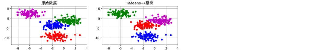
plt.figure(figsize=(9, 10), facecolor='w')
    plt.subplot(421)
    plt.title(u'原始数据')
    plt.scatter(data[:, 0], data[:, 1], c=y, s=30, cmap=cm, edgecolors='none')
    x1_min, x2_min = np.min(data, axis=0)
    x1_max, x2_max = np.max(data, axis=0)
    x1_min, x1_max = expand(x1_min, x1_max)
    x2_min, x2_max = expand(x2_min, x2_max)
    plt.xlim((x1_min, x1_max))
    plt.ylim((x2_min, x2_max))
    plt.grid(True)

    plt.subplot(422)
    plt.title(u'KMeans++聚类')
    plt.scatter(data[:, 0], data[:, 1], c=y_hat, s=30, cmap=cm, edgecolors='none')
    plt.xlim((x1_min, x1_max))
    plt.ylim((x2_min, x2_max))
    plt.grid(True)
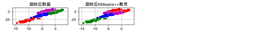
    plt.subplot(423)
    plt.title(u'旋转后数据')
    plt.scatter(data_r[:, 0], data_r[:, 1], c=y, s=30, cmap=cm, edgecolors='none')
    x1_min, x2_min = np.min(data_r, axis=0)
    x1_max, x2_max = np.max(data_r, axis=0)
    x1_min, x1_max = expand(x1_min, x1_max)
    x2_min, x2_max = expand(x2_min, x2_max)
    plt.xlim((x1_min, x1_max))
    plt.ylim((x2_min, x2_max))
    plt.grid(True)

    plt.subplot(424)
    plt.title(u'旋转后KMeans++聚类')
    plt.scatter(data_r[:, 0], data_r[:, 1], c=y_r_hat, s=30, cmap=cm, edgecolors='none')
    plt.xlim((x1_min, x1_max))
    plt.ylim((x2_min, x2_max))
    plt.grid(True)
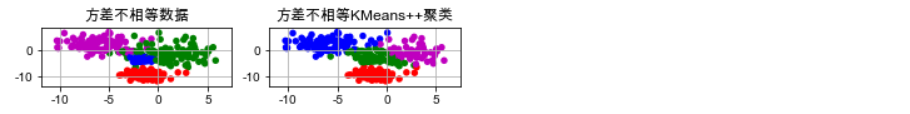
    plt.subplot(425)
    plt.title(u'方差不相等数据')
    plt.scatter(data2[:, 0], data2[:, 1], c=y2, s=30, cmap=cm, edgecolors='none')
    x1_min, x2_min = np.min(data2, axis=0)
    x1_max, x2_max = np.max(data2, axis=0)
    x1_min, x1_max = expand(x1_min, x1_max)
    x2_min, x2_max = expand(x2_min, x2_max)
    plt.xlim((x1_min, x1_max))
    plt.ylim((x2_min, x2_max))
    plt.grid(True)

    plt.subplot(426)
    plt.title(u'方差不相等KMeans++聚类')
    plt.scatter(data2[:, 0], data2[:, 1], c=y2_hat, s=30, cmap=cm, edgecolors='none')
    plt.xlim((x1_min, x1_max))
    plt.ylim((x2_min, x2_max))
    plt.grid(True)
    plt.subplot(427)
    plt.title(u'数量不相等数据')
    plt.scatter(data3[:, 0], data3[:, 1], s=30, c=y3, cmap=cm, edgecolors='none')
    x1_min, x2_min = np.min(data3, axis=0)
    x1_max, x2_max = np.max(data3, axis=0)
    x1_min, x1_max = expand(x1_min, x1_max)
    x2_min, x2_max = expand(x2_min, x2_max)
    plt.xlim((x1_min, x1_max))
    plt.ylim((x2_min, x2_max))
    plt.grid(True)

    plt.subplot(428)
    plt.title(u'数量不相等KMeans++聚类')
    plt.scatter(data3[:, 0], data3[:, 1], c=y3_hat, s=30, cmap=cm, edgecolors='none')
    plt.xlim((x1_min, x1_max))
    plt.ylim((x2_min, x2_max))
    plt.grid(True)

    plt.tight_layout(2)
    plt.suptitle(u'数据分布对KMeans聚类的影响', fontsize=18)
    plt.subplots_adjust(top=0.92)
    plt.show()


5 总结
5.1 聚类的各种方式

5.2 K-Means算法的实现步骤

6 笔面试相关
6.1 聚类的基本问题有哪些?
性能度量和距离计算
6.2 K-Means聚类的伪代码?
