1、灰度变换
1)灰度图的线性变换
Gnew = Fa * Gold + Fb。
Fa为斜线的斜率,Fb为y轴上的截距。
Fa>1 输出图像的对比度变大,否则变小。
Fa=1 Fb≠0时,图像的灰度上移或下移,效果为图像变亮或变暗。
Fa=-1,Fb=255时,发生图像反转。
注意:线性变换会出现亮度饱和而丢失细节。
2)对数变换
t=c * log(1+s)
c为变换尺度,s为源灰度,t为变换后的灰度。
对数变换自变量低时曲线斜率高,自变量大时斜率小。所以会放大图像较暗的部分,压缩较亮的部分。
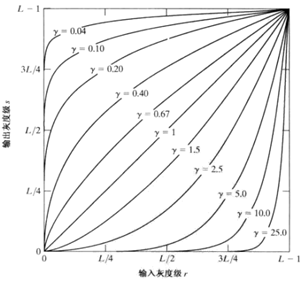
3)伽马变换
y=(x+esp)γ,x与y的范围是[0,1], esp为补偿系数,γ为伽马系数。
当伽马系数大于1时,图像高灰度区域得到增强。
当伽马系数小于1时,图像低灰度区域得到增强。
当伽马系数等于1时,图像线性变换。
4)图像取反
方法1:直接取反
imgPath = 'E:opencv_picsrc_picpic2.bmp';
img1 = imread(imgPath); % 前景图
img0 = 255-img1; % 取反景图
subplot(1,2,1),imshow(img1),title('原始图像');
subplot(1,2,2),imshow(img0),title('取反图像');

方法2:伽马变换
Matlab:imadjust(f, [low_in, high_in], [low_out, high_out], gamma)
[low_in, high_in]范围内的数据映射到 [low_out, high_out],低于low的映射到low_out, 高于high的映射到high_out.
imgPath = 'E:opencv_picsrc_picpic2.bmp';
img1 = imread(imgPath); % 前景图
img0 = imadjust(img1, [0,1], [1,0]);
subplot(1,2,1),imshow(img1),title('原始图像');
subplot(1,2,2),imshow(img0),title('取反图像');

2、二值化
1)rgb2gray
一般保存的灰度图是24位的灰度,如果改为8bit灰度图。则可以用rgb2gray函数。
img= rgb2gray(img);
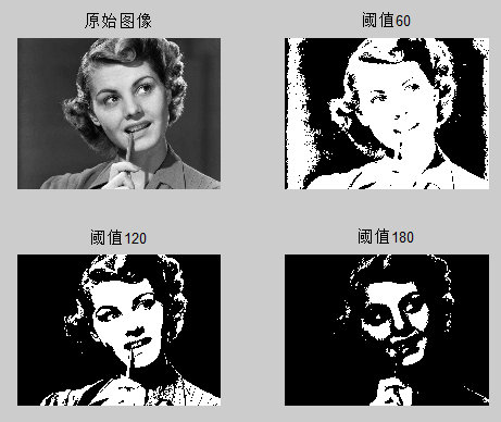
2)Matlab使用比较运算符二值化
imgPath = 'E:opencv_picsrc_picpic4.bmp';
img = imread(imgPath); % 前景图
img = rgb2gray(img);
img1 = img > 60;
img2 = img > 120;
img3 = img > 180;
subplot(2,2,1),imshow(img), title('原始图像');
subplot(2,2,2),imshow(img1),title('阈值60');
subplot(2,2,3),imshow(img2),title('阈值120');
subplot(2,2,4),imshow(img3),title('阈值180');
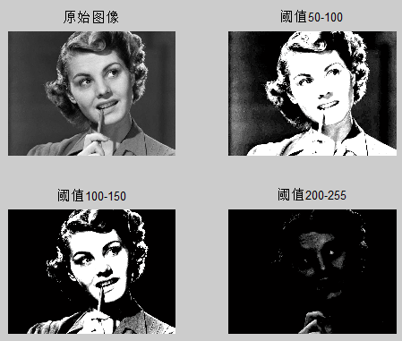
3)imshow参数指定图像灰度范围
imshow函数显示图片时,可以指定灰度等级。
imshow(img, [100,150])
小于100的直接设置为黑色,大于150的直接设置为白色。二者之间的设置为中等亮度。
imshow(img, [100,101])就可以实现二值化,图像分界线在100。
imgPath = 'E:opencv_picsrc_picpic4.bmp';
img = imread(imgPath);
img= rgb2gray(img);

subplot(2,2,1),imshow(img), title('原始图像');
subplot(2,2,2),imshow(img,[50,100]),title('阈值50-100');
subplot(2,2,3),imshow(img, [100, 150]),title('阈值100-150');
subplot(2,2,4),imshow(img,[200,255]),title('阈值200-255');
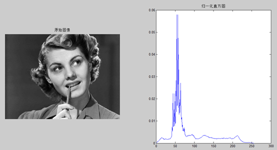
3、灰度直方图
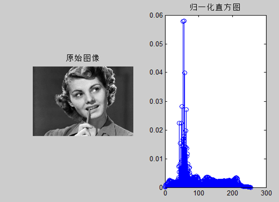
灰度直方图:横坐标是灰度,纵坐标是该灰度在图像中出现的次数。
归一化直方图,纵坐标对应着该灰度级别在图像中出现的概率。
subplot(1,2,1),imshow(img), title('原始图像');
subplot(1,2,2),imhist(img),title('直方图');

绘制归一化直方图。
subplot(1,2,1),imshow(img), title('原始图像');
subplot(1,2,2),p = imhist(img)/numel(img) ;
plot(p), title('归一化直方图');
或者使用stem函数绘制归一化直方图。
subplot(1,2,1),imshow(img), title('原始图像');
[count,x] = imhist(img);
[m,n]=size(img);
count = count/(m*n);
subplot(1,2,2), stem(x, count) , title('归一化直方图');
img = img > 100;
subplot(1,2,1),imshow(img), title('原始图像');
subplot(1,2,2),imhist(img), title('直方图');
把图片转换为二值化图像,直方图如下。灰度只有0和1,符合二值化图的特点。

对这个直方图归一化,因为是二值化的图,所以归一化后就是个子的比例。
p = imhist(img)/numel(img)
p =
0.6980
0.3020
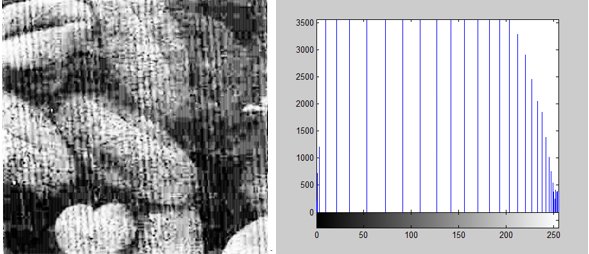
Imhist(img,b); 可以指定灰度等级b,默认是256级,实际工程中一般32级,如下图。

4、直方图均衡化
直方图均衡化即灰度均衡化,通过灰度映射,使输入图像的灰度转换为在每一级灰度上都有近似相同的点数分布,这样输出的直方图就是均匀的,图像获得较高的对比度和较大的动态范围。
直方图均衡化对图像进行非线性拉伸,重新分配图像像素值,使一定灰度范围内的像素数量大致相同。使用直方图均衡化技术来处理图像,能扩展图像的动态范围,扩宽灰度等级范围,提高对比度。
histeq(img,b);%b是灰度等级。2级均衡化就是二值化。
subplot(1,4,1),imshow(img), title('原始图像');
subplot(1,4,2),histeq(img, 2), title('2级直方图均衡化');
subplot(1,4,3),histeq(img, 32), title('32级直方图均衡化');
subplot(1,4,4),histeq(img), title('255级直方图均衡化');
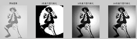
可见直方图均衡化之后,图像亮度变得均匀,提高了对比度。
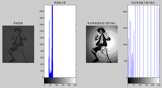
调用img=img*0.3;调暗了图像,再次均衡化,图像的效果没有发生改变,可见均衡化可以用作图像处理前把图像转为统一的形式。

下图是imhist(img)之后的直方图。可见histeq将图划分灰度等级获得比较均匀平坦的直方图。
subplot(1,4,1),imshow(img), title('原始图像');
subplot(1,4,2),imhist(img), title('原图直方图');

subplot(1,4,3),imshow(histeq(img)), title('降低亮度图后直方图均衡化');
subplot(1,4,4),imhist(histeq(img)), title('降低亮度直方图均衡化');
再举一个例子,直方图均衡化调整较暗的图片。
图片较暗,动态范围低。直方图灰度等级偏暗,在高亮度区域分配像素很少。
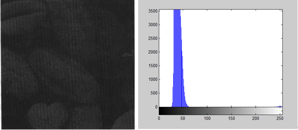
使用均衡化处理,然后显示,直方图各个灰度等级的数据较均匀。
g=histeq(img, 256);
imshow(g)
尊重原创技术文章,转载请注明。