20181202 2019-2020-2 《Python程序设计》实验四报告

20181202 2019-2020-2 《Python程序设计》实验四Python综合实践

课程：《Python程序设计》
班级： 20181202
姓名：李祎铭
学号：20181202
实验教师：王志强
实验日期：2020年6月1日
必修/选修：公选课

1.实验内容

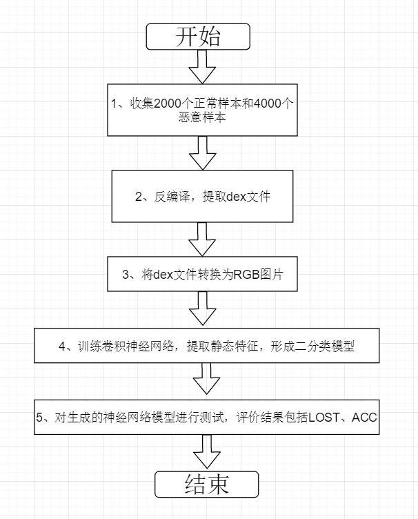
此实验为我学习深度学习的第一部分内容：主要目标是学习基础知识、Keras框架简单应用、数据集构建，同时为解决实际问题提出简易方案。

在下一阶段的学习中我将进行刚深入的学习，主要依靠Paddle框架和Tensorflow框架完成更加完善且具有现实意义的程序。

2. 实验过程及结果

此处填写实验的过程及结果

配置科学计算工作环境

Anaconda(包含numpy)
Keras
Theano
Pycharm

数据集构建

安卓应用APK安装包反编译
提取dex特征文件
dex文件转换为图片

训练卷积神经网络

使用Keras架构构建简易卷积神经网络
训练分类模型

3. 实验过程中遇到的问题和解决过程

PART1配置科学计算工作环境

首先你需要有pycharm(或者其他的你喜欢用的IDE)
在安装Anaconda之前你最好删除(彻底)你原有的python环境，Anaconda是一个开源的python发行版本，其中包含了主流的科学计算库，我将其理解为python plus

Anaconda官网下载，下载安装没什么可说的
安装好Anaconda后一定要记得配置环境变量
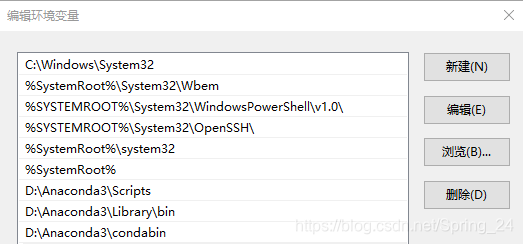
配置好环境变量之后启动Anaconda Prompt，安装gcc环境,只有在配置好gcc环境后numpy的数组操作才不会报错

conda update conda
conda install libpython
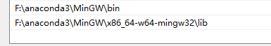
conda install mingw

这之后要记得将MinGW加入到环境变量

之后安装theano和Keras(简单的pip指令即可)

pip install theano
pip install keras

至此使用CPU的计算环境配置完成，后续代码中的使用库可以同样的方法安装

conda install xxx
pip install xxx
```python
import os
import zipfile

path="/home/chicho/test/test/"  # this is apk files' store path
dex_path="/home/chicho/test/test/dex/" # a directory  store dex files 
 
apklist = os.listdir(path) # get all the names of apps
 
if not os.path.exists(dex_path):
    os.makedirs(dex_path)
 
for APK in apklist:
    portion = os.path.splitext(APK)
 
    if portion[1] == ".apk":
        newname = portion[0] + ".zip" # change them into zip file to extract dex files
 
        os.rename(APK,newname)
 
    if APK.endswith(".zip"):
        apkname = portion[0]
 
        zip_apk_path = os.path.join(path,APK) # get the zip files
 
        z = zipfile.ZipFile(zip_apk_path, 'r') # read zip files
 
        for filename in z.namelist():
            if filename.endswith(".dex"):
                dexfilename = apkname + ".dex"
                dexfilepath = os.path.join(dex_path, dexfilename)
                f = open(dexfilepath, 'w+') # eq: cp classes.dex dexfilepath
                f.write(z.read(filename))

print("all work done!")
---
### ==PART2数据集构建==
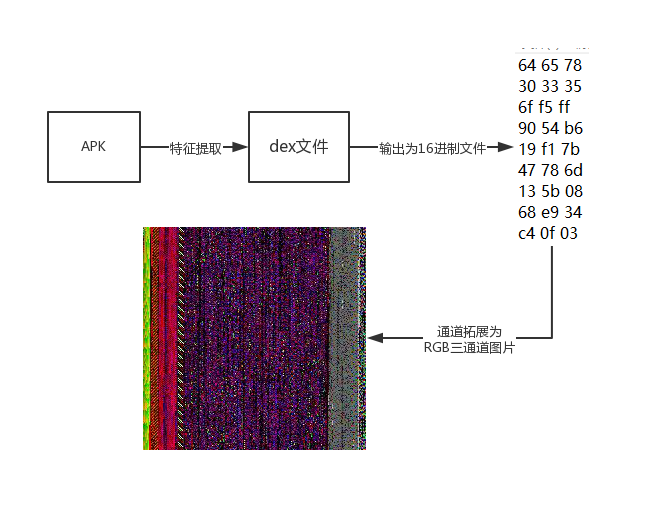
1. 首先利用反编译技术提取出APK文件中的dex文件，原理很简单，就是目录遍历加解压缩，直接上代码

``` python

为了实现检测安卓恶意应用，我需要实现将dex文件转换为RGB三通道彩色图像图像，每个图象都形如：

[[255,255,255] [255,255,255] [255,255,255] 
[255,255,255] [255,255,255] [255,255,255] 
[255,255,255] [255,255,255] [255,255,255] 
[255,255,255] [255,255,255] [255,255,255] 
...
]

不是n维数组，是numpy数组，所以没有逗号间隔
我的设计思路如图：

代码如下：

# coding: utf-8
# !/usr/bin/env python
# encoding: utf-8coding: utf-8
# 不含0x
# 程序目标，读取dex，然后以16进制方式写到txt文件
from PIL import Image
import re
import math
import os

# count = len(open('classes_dex_denary_three.txt','rU').readlines())

dex_path = r"D:45"  # a directory  store dex files
dexlist = os.listdir(dex_path)  # get all the names of dex

txt_path = r"D:45txt"  # a directory  store txt files

rgb_path = r"D:45jpg"  # a directory  store rgb files


def main():
    for dexfile in dexlist:
        if dexfile.endswith(".dex"):
            f3 = open(dexfile, "rb")
            portion = os.path.splitext(dexfile)
            txtfilename = portion[0] + ".txt"
            txtfilepath = os.path.join(txt_path, txtfilename)
            outfile = open(txtfilepath, "wb")
            i = 0
            res=""
            while 1:
                c = f3.read(1)
                i = i + 1
                if not c:
                    break
                if i % 4 == 0:
                    outfile.write(("
").encode())
                else:
                    if ord(c) <= 15:
                        res=("0x0" + hex(ord(c))[2:])[2:] + " "
                        outfile.write(res.encode())
                    else:
                        res=(hex(ord(c)))[2:] + " "
                        outfile.write(res.encode())
            outfile.close()
            f3.close()


if __name__ == "__main__":
    main()

txtlist = os.listdir(txt_path)  # get all the names of txt
# rgblist = os.listdir(rgb_path) # get all the names of rgb
for txtfile in txtlist:
    if txtfile.endswith(".txt"):
        txtportion = os.path.splitext(txtfile)
        rgbfilename = txtportion[0] + ".jpg"
        rgbfilepath = os.path.join(rgb_path, rgbfilename)
        count = -1
        txtfilepath = os.path.join(txt_path, txtfile)
        for count, line in enumerate(open(txtfilepath, 'r')):
            pass
        count += 1
        x = int(math.sqrt(count - 1))
        y = int(math.sqrt(count - 1))
        image = Image.new("RGB", (x, y))
        f4 = open(txtfilepath, 'rb')
        for i in range(0, x):
            for j in range(0, y):
                line = f4.readline()
                rgbvalue = line.split((" ").encode())
                image.putpixel((i, j), (int(rgbvalue[0], 16), int(rgbvalue[1], 16), int(rgbvalue[2], 16)))
        image.save(rgbfilepath)
        f4.close()
# print(count)
print("all work done!")

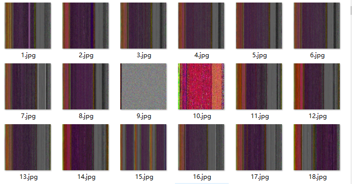
至此我就得到了一整个充满jpg图片的数据集

PART3训练卷积神经网络

如果你觉得我写的不够详细可以参考这篇博客
受限于时间和难度，我选择了较为简单的Keras框架，但在下一阶段我会从更底层的问题开始考虑使用更高级也相对复杂的框架
训练流程图

源代码中的文件结构

dataset

malware
static

pyimagesearch

pycache
init.py
CNN.py

tools

d2j.py
dex_extract.py
zip.py

train.py
lb.pickle
malware.model
plot.png

dateset中的文件包含两类图片数据集
pyimagesearch中包含卷积神经网络的结构模型
tools中包含将APK文件批量提取特征并转化为jpg图片的程序
train.py训练神经网络的启动程序
lb.pickle训练生成的二分类
malware.model训练生成的模型
plot.png训练准确度图像

首先是CNN结构模型,采取的是5层结构神经网络结构，即：卷积层(Conv2D)->池化层(MaxPooling2D)->卷积层(Conv2D)->池化层(MaxPooling2D)->全连接层()

import os
os.environ['KERAS_BACKEND']='theano'
from keras.models import Sequential
from keras.layers.normalization import BatchNormalization
from keras.layers.convolutional import Conv2D
from keras.layers.convolutional import MaxPooling2D
from keras.layers.core import Activation
from keras.layers.core import Flatten
from keras.layers.core import Dropout
from keras.layers.core import Dense
from keras import backend as K

class SmallerVGGNet:
	@staticmethod
	def build(width, height, depth, classes):
		# initialize the model along with the input shape to be
		# "channels last" and the channels dimension itself
		model = Sequential()
		inputShape = (height, width, depth)
		chanDim = -1

		# if we are using "channels first", update the input shape
		# and channels dimension
		if K.image_data_format() == "channels_first":
			inputShape = (depth, height, width)
			chanDim = 1

					# CONV => RELU => POOL
		model.add(Conv2D(32, (3, 3), padding="same",
			input_shape=inputShape))
		model.add(Activation("relu"))
		model.add(BatchNormalization(axis=chanDim))
		model.add(MaxPooling2D(pool_size=(3, 3)))
		model.add(Dropout(0.25))

				# (CONV => RELU) * 2 => POOL
		model.add(Conv2D(128, (3, 3), padding="same"))
		model.add(Activation("relu"))
		model.add(BatchNormalization(axis=chanDim))
		model.add(Conv2D(128, (3, 3), padding="same"))
		model.add(Activation("relu"))
		model.add(BatchNormalization(axis=chanDim))
		model.add(MaxPooling2D(pool_size=(2, 2)))
		model.add(Dropout(0.25))

		# first (and only) set of FC => RELU layers
		model.add(Flatten())
		model.add(Dense(1024))
		model.add(Activation("relu"))
		model.add(BatchNormalization())
		model.add(Dropout(0.5))

		# softmax classifier
		model.add(Dense(classes))
		model.add(Activation("softmax"))

		# return the constructed network architecture
		return model

训练程序train.py

# set the matplotlib backend so figures can be saved in the background
import os
os.environ['KERAS_BACKEND']='theano'
from keras.utils import to_categorical


import matplotlib
matplotlib.use("Agg")

# import the necessary packages
from keras.preprocessing.image import ImageDataGenerator
from keras.optimizers import Adam
from keras.preprocessing.image import img_to_array
from sklearn.preprocessing import LabelBinarizer
from sklearn.model_selection import train_test_split
from pyimagesearch.CNN import SmallerVGGNet
import matplotlib.pyplot as plt
from imutils import paths
import numpy as np
import argparse
import random
import pickle
import cv2
import os

# construct the argument parse and parse the arguments
ap = argparse.ArgumentParser()
ap.add_argument("-d", "--dataset", required=True,
	help="path to input dataset (i.e., directory of images)")
ap.add_argument("-m", "--model", required=True,
	help="path to output model")
ap.add_argument("-l", "--labelbin", required=True,
	help="path to output label binarizer")
ap.add_argument("-p", "--plot", type=str, default="plot.png",
	help="path to output accuracy/loss plot")
args = vars(ap.parse_args())

# initialize the number of epochs to train for, initial learning rate,
# batch size, and image dimensions
EPOCHS = 100
INIT_LR = 1e-3
BS = 32
IMAGE_DIMS = (96, 96, 3)

# initialize the data and labels
data = []
labels = []

# grab the image paths and randomly shuffle them
print("[INFO] loading images...")
imagePaths = sorted(list(paths.list_images(args["dataset"])))
random.seed(42)
random.shuffle(imagePaths)

# loop over the input images
for imagePath in imagePaths:
	# load the image, pre-process it, and store it in the data list
	image = cv2.imread(imagePath)
	image = cv2.resize(image, (IMAGE_DIMS[1], IMAGE_DIMS[0]))
	image = img_to_array(image)
	data.append(image)

	# extract the class label from the image path and update the
	# labels list
	label = imagePath.split(os.path.sep)[-2]
	labels.append(label)

# scale the raw pixel intensities to the range [0, 1]
data = np.array(data, dtype="int16") / 255.0
labels = np.array(labels)
print("[INFO] data matrix: {:.2f}MB".format(
	data.nbytes / (1024 * 1000.0)))

# binarize the labels
lb = LabelBinarizer()
labels = lb.fit_transform(labels)
labels = to_categorical(labels) #one-hot

# partition the data into training and testing splits using 80% of
# the data for training and the remaining 20% for testing
(trainX, testX, trainY, testY) = train_test_split(data,
	labels, test_size=0.2, random_state=42)

# construct the image generator for data augmentation
aug = ImageDataGenerator(rotation_range=25, width_shift_range=0.1,
	height_shift_range=0.1, shear_range=0.2, zoom_range=0.2,
	horizontal_flip=True, fill_mode="nearest")

# initialize the model
print("[INFO] compiling model...")
model = SmallerVGGNet.build(width=IMAGE_DIMS[1], height=IMAGE_DIMS[0],
	depth=IMAGE_DIMS[2], classes=len(lb.classes_))
opt = Adam(lr=INIT_LR, decay=INIT_LR / EPOCHS)
model.compile(loss="binary_crossentropy", optimizer=opt,
	metrics=["accuracy"])

# train the network
print("[INFO] training network...")
H = model.fit_generator(
	aug.flow(trainX, trainY, batch_size=BS),
	validation_data=(testX, testY),
	steps_per_epoch=len(trainX) // BS,
	epochs=EPOCHS, verbose=1)

# save the model to disk
print("[INFO] serializing network...")
model.save(args["model"])

# save the label binarizer to disk
print("[INFO] serializing label binarizer...")
f = open(args["labelbin"], "wb")
f.write(pickle.dumps(lb))
f.close()

# plot the training loss and accuracy
plt.style.use("ggplot")
plt.figure()
N = EPOCHS
plt.plot(np.arange(0, N), H.history["loss"], label="train_loss")
plt.plot(np.arange(0, N), H.history["val_loss"], label="val_loss")
plt.plot(np.arange(0, N), H.history["accuracy"], label="train_acc")
plt.plot(np.arange(0, N), H.history["val_accuracy"], label="val_acc")
plt.title("Training Loss and Accuracy")
plt.xlabel("Epoch #")
plt.ylabel("Loss/Accuracy")
plt.legend(loc="upper left")
plt.savefig(args["plot"])

启动训练

python train.py --dataset dataset --model malware.model --labelbin lb.pickle
左侧为训练过程，右侧是利用可视化技术生成的准确度图像

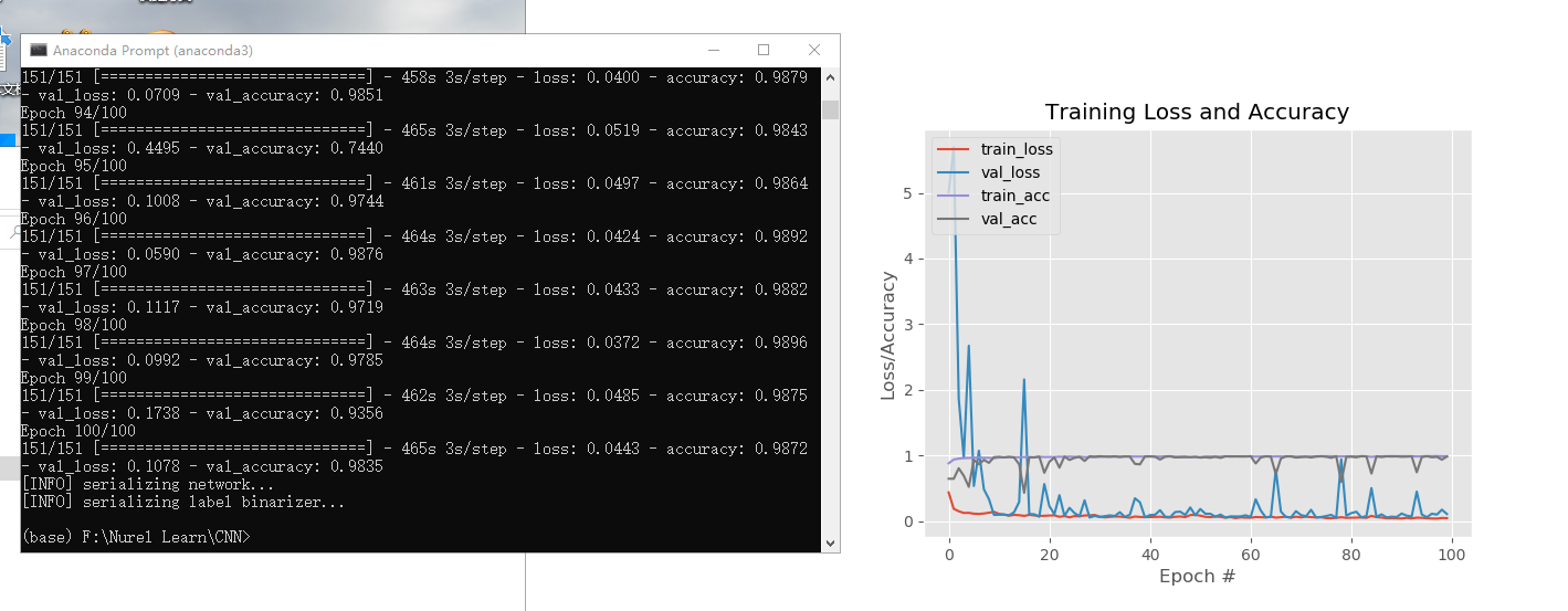
模型性能(准确率)
该测试部分主要包含ACC（准确率）、val_ACC（过程准确率）、LOST（丢失率）、val_LOST（过程丢失率）指标。各项指标的具体概念如下：
通过在训练中，将一部分输入图像设定为测试图像来评价每一轮训练的准确率和丢失率。

ACC
即精确率，描述最终模型预测的准确率。
val_ACC
即过程精确率，描述在一轮训练中模型预测的准确率。
LOST
即丢失率，描述最终模型预测的丢失率。
val_LOST
即过程丢失率，描述在一轮训练中模型预测的丢失率。

从最终的训练中我们可以看到这个模型的准确度达到了98%以上，可以说是非常准确了

其他（感悟、思考等）

上了一学期python程序设计课，以及学了两年python的一点感受

python很方便，真的很方便，库多涵盖面广，使用最多的可视化、网络编程、人工智能等等功能都非常齐全，当然python对程序员友好的背后就是对机器的不友好，运行速度慢是必然的，无论是在我初学python的时候还是在开始深入学习python的时候，总是看到说python效率低的人。但是，大家仍然在用python做着人工智能、爬虫、数据可视化等等，这就足以说明python所具有的活力，学python稳赚不赔！！
在这里我就不单独列举我学了什么、领悟了什么，只想再讲一下下一阶段的学习目标。在接下来的学习中我想完成这样两件事情：1.将python与我专业所学知识结合起来，用python程序简化复杂的工作流程；2.深入学习人工智能，短短一个月的学习我仅仅看到了人工智能的冰山一角，我想继续深入学习，成就更好的自己。

20181202 2019-2020-2 《Python程序设计》 实验四报告

20181202 2019-2020-2 《Python程序设计》实验四Python综合实践

1.实验内容

2. 实验过程及结果

3. 实验过程中遇到的问题和解决过程

PART1配置科学计算工作环境

PART3训练卷积神经网络

其他（感悟、思考等）

上了一学期python程序设计课，以及学了两年python的一点感受

20181202 2019-2020-2 《Python程序设计》实验四报告