1. 高斯牛顿法
残差函数f(x)为非线性函数,对其一阶泰勒近似有:
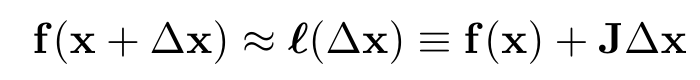
这里的J是残差函数f的雅可比矩阵,带入损失函数的:
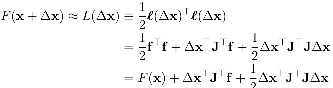

令其一阶导等于0,得:
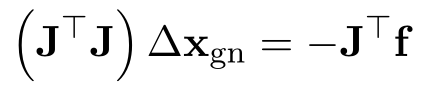
这就是论文里常看到的normal equation。
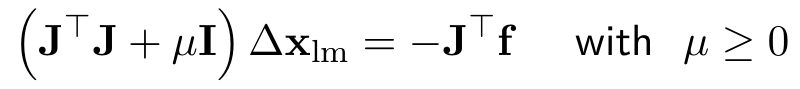
2.LM
LM是对高斯牛顿法进行了改进,在求解过程中引入了阻尼因子:
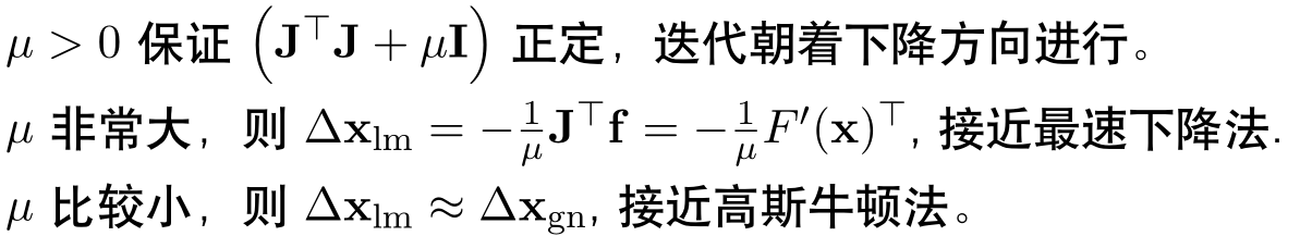
2.1 阻尼因子的作用:
2.2 阻尼因子的初始值选取:
一个简单的策略就是: 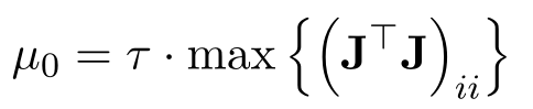
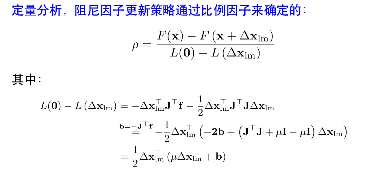
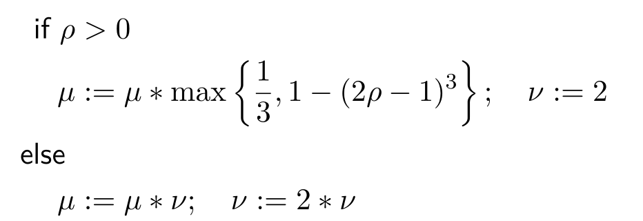
2.3 阻尼因子的更新策略

3.核心代码讲解
3.1 构建H矩阵
void Problem::MakeHessian() {
    TicToc t_h;
    // 直接构造大的 H 矩阵
    ulong size = ordering_generic_;
    MatXX H(MatXX::Zero(size, size));
    VecX b(VecX::Zero(size));

    // TODO:: accelate, accelate, accelate
//#ifdef USE_OPENMP
//#pragma omp parallel for
//#endif

    // 遍历每个残差,并计算他们的雅克比,得到最后的 H = J^T * J
    for (auto &edge: edges_) {

        edge.second->ComputeResidual();
        edge.second->ComputeJacobians();

        auto jacobians = edge.second->Jacobians();
        auto verticies = edge.second->Verticies();
        assert(jacobians.size() == verticies.size());
        for (size_t i = 0; i < verticies.size(); ++i) {
            auto v_i = verticies[i];
            if (v_i->IsFixed()) continue;    // Hessian 里不需要添加它的信息,也就是它的雅克比为 0

            auto jacobian_i = jacobians[i];
            ulong index_i = v_i->OrderingId();
            ulong dim_i = v_i->LocalDimension();

            MatXX JtW = jacobian_i.transpose() * edge.second->Information();
            for (size_t j = i; j < verticies.size(); ++j) {
                auto v_j = verticies[j];

                if (v_j->IsFixed()) continue;

                auto jacobian_j = jacobians[j];
                ulong index_j = v_j->OrderingId();
                ulong dim_j = v_j->LocalDimension();

                assert(v_j->OrderingId() != -1);
                MatXX hessian = JtW * jacobian_j;
                // 所有的信息矩阵叠加起来
                H.block(index_i, index_j, dim_i, dim_j).noalias() += hessian;
                if (j != i) {
                    // 对称的下三角
                    H.block(index_j, index_i, dim_j, dim_i).noalias() += hessian.transpose();
                }
            }
            b.segment(index_i, dim_i).noalias() -= JtW * edge.second->Residual();
        }

    }
    Hessian_ = H;
    b_ = b;
    t_hessian_cost_ += t_h.toc();

    delta_x_ = VecX::Zero(size);  // initial delta_x = 0_n;

}
3.2 将构建好的H矩阵加上阻尼因子
void Problem::AddLambdatoHessianLM() {
    ulong size = Hessian_.cols();
    assert(Hessian_.rows() == Hessian_.cols() && "Hessian is not square");
    for (ulong i = 0; i < size; ++i) {
        Hessian_(i, i) += currentLambda_;
    }
}
3.3 进行求解后,验证该步的解是否合适,代码对应阻尼因子的更新策略
bool Problem::IsGoodStepInLM() {
    double scale = 0;
    scale = delta_x_.transpose() * (currentLambda_ * delta_x_ + b_);
    scale += 1e-3;    // make sure it's non-zero :)

    // recompute residuals after update state
    // 统计所有的残差
    double tempChi = 0.0;
    for (auto edge: edges_) {
        edge.second->ComputeResidual();
        tempChi += edge.second->Chi2();
    }

    double rho = (currentChi_ - tempChi) / scale;
    if (rho > 0 && isfinite(tempChi))   // last step was good, 误差在下降
    {
        double alpha = 1. - pow((2 * rho - 1), 3);
        alpha = std::min(alpha, 2. / 3.);
        double scaleFactor = (std::max)(1. / 3., alpha);
        currentLambda_ *= scaleFactor;
        ni_ = 2;
        currentChi_ = tempChi;
        return true;
    } else {
        currentLambda_ *= ni_;
        ni_ *= 2;
        return false;
    }
}