
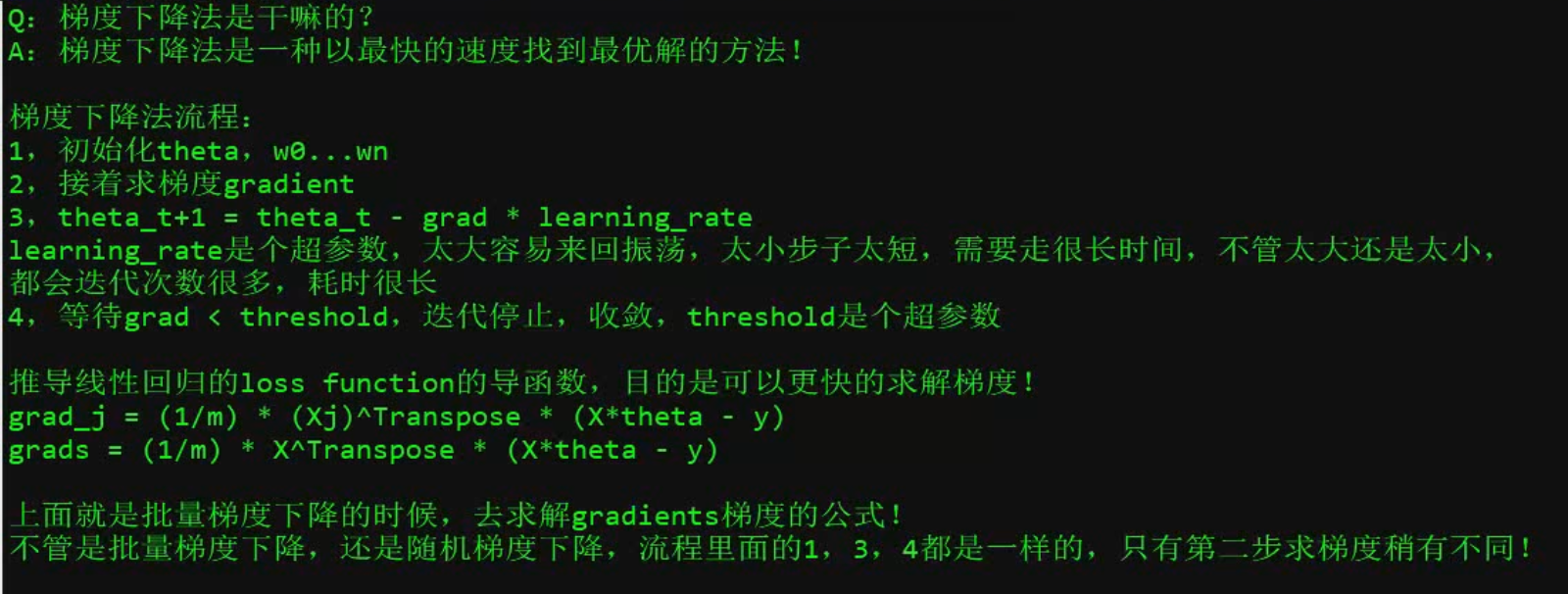
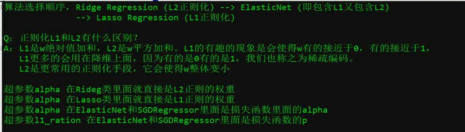
正态分布

import numpy as np  #数学计算的框架
import matplotlib.pyplot as plt #绘图的框架

#这里相当于是随即X维度X1,rand是随机均匀分布
X=2*np.random.rand(100,1)#rand返回100行1列[0,1)   均匀分布

#人为的设置真是的Y一列,randn是设置error,ranndn是标准正态分布
Y=4+3*X+np.random.randn(100,1)   #randn    标准正态分布     #4*X0(X0为1嘛)+3*X 看成预测值   np.random.randn(100,1)看成随机误差【独立服从正态分布,这里用标准正态分布模拟】
#整合X0与X1 #numpy.c_(就是英文单词conbine的意思)
X_b=np.c_[np.ones((100,1)),X]
# print(X_b)

#linalg线性代数 inv(inverse)求逆  .T就是转置  .dot(点乘 进行矩阵运算)
theta_best=np.linalg.inv(X_b.T.dot(X_b)).dot(X_b.T).dot(Y)
print(theta_best)
#theta_best  2行1列
#可以知道包括X0在内有几组X的值,W0~~Wn即theta_best就有几行1列的值

#创建测试机里面的X1
X_new=np.array([[0],[2]])
X_new_b=np.c_[(np.ones((2,1))),X_new] #n行2列
# print(X_new_b)
y_predict=X_new_b.dot(theta_best)
print(y_predict)

plt.plot(X_new,y_predict,'r-')#红色用-绘图  预测值
plt.plot(X,Y,'b.')#蓝色用.绘制     实际值
plt.axis([0,2,0,15])#X轴范围0-2  Y轴范围0-15
plt.show()
使用sklearn
import numpy as np
from sklearn.linear_model import LinearRegression #线性回归
import matplotlib.pyplot as plt
X=2*np.random.rand(100,1)#rand返回100行1列[0,1)   均匀分布
Y=4+3*X+np.random.randn(100,1)

lin_reg=LinearRegression()
#fit 训练 这个方法指的研究
lin_reg.fit(X,Y)
#intercept_截距W0  coef_其他的参数W1~Wn
print(lin_reg.intercept_,lin_reg.coef_)

#使用predict去预测
X_new=np.array([[0],[2]])
print(lin_reg.predict(X_new))
import numpy as np

X=2*np.random.rand(100,1) #均匀分布取100,1向量
Y=4+3*X+np.random.randn(100,1) #标准正态分布,取得Y值
X_b=np.c_[np.ones((100,1)),X] #拼接X矩阵,每行的X0都是1

learning_rate=0.1    #学习绿
n_iterations=10000#设置最大迭代次数
m=100#样本数 为了loss取平均,否则我数据量大的话loss反而大,不对,我要知道平均是不是大,就是把100 和 1000统一来看意思

theta=np.random.randn(2,1)#2因为X_b初始化俩个维度
count=0#当前迭代次数

for iteration in range(n_iterations):
    count+=1
    gradients=1/m*X_b.T.dot(X_b.dot(theta)-Y)#各个点位的斜率
    # print(gradients)
    theta=theta-learning_rate*gradients#theta赋予此次迭代的值
    # print(gradients)
print(count)
print(theta)


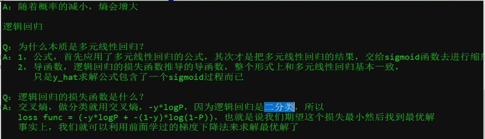
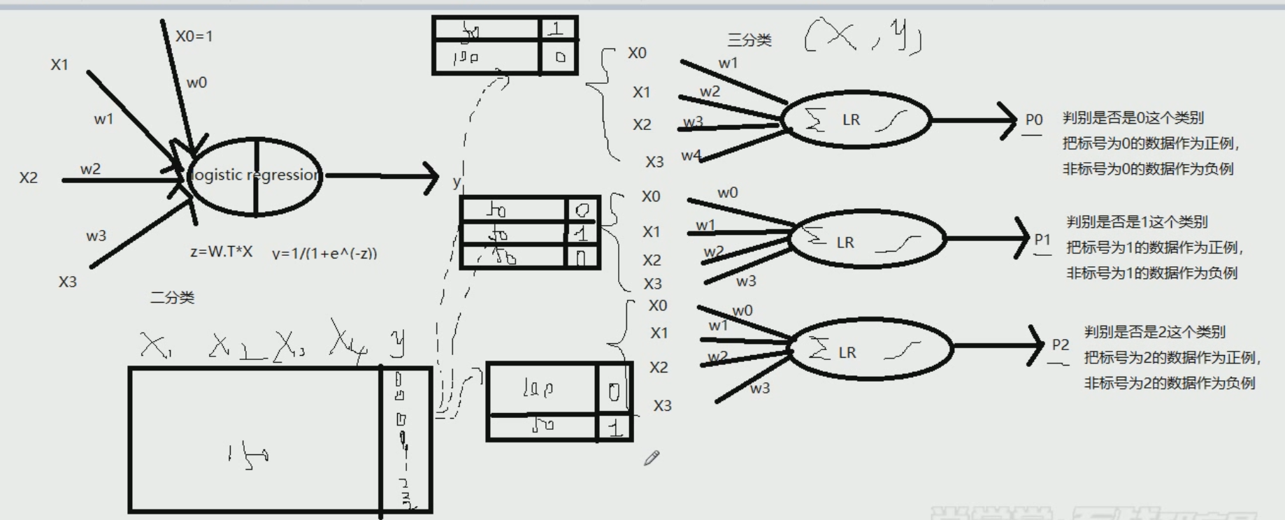
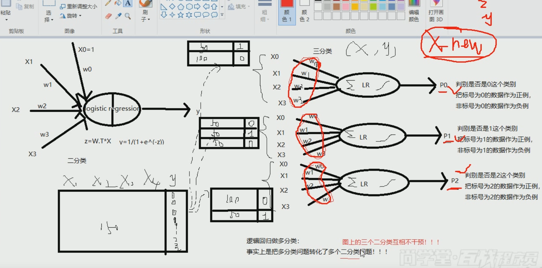
逻辑回归分析过程~~~~~
傅里叶变换:将时间轴拆分将频率分别分解出来,然后从侧面审视这些频率
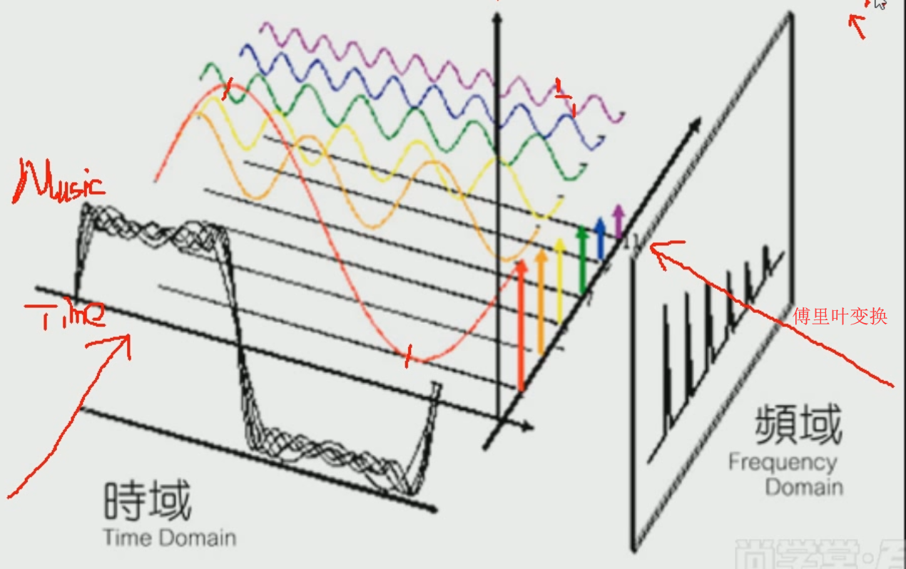
HZ太高就成噪声了,因此我们可以将维,比如就取前3000HZ
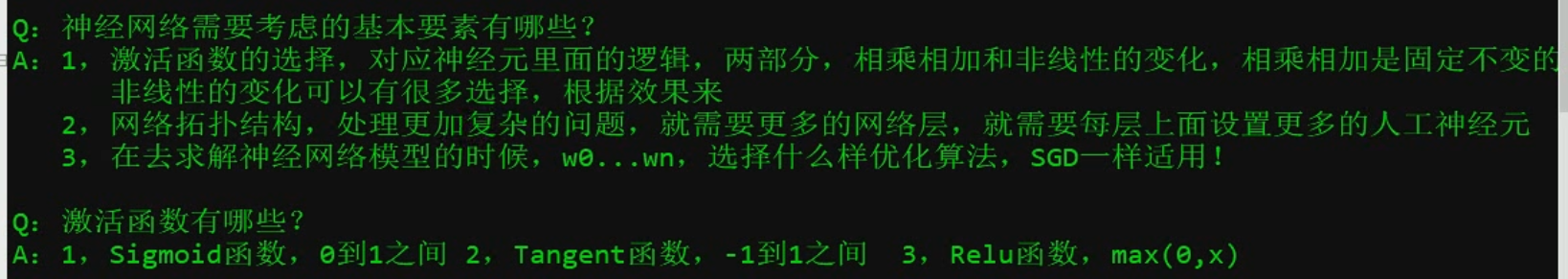
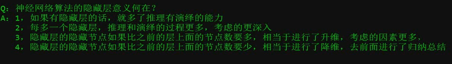
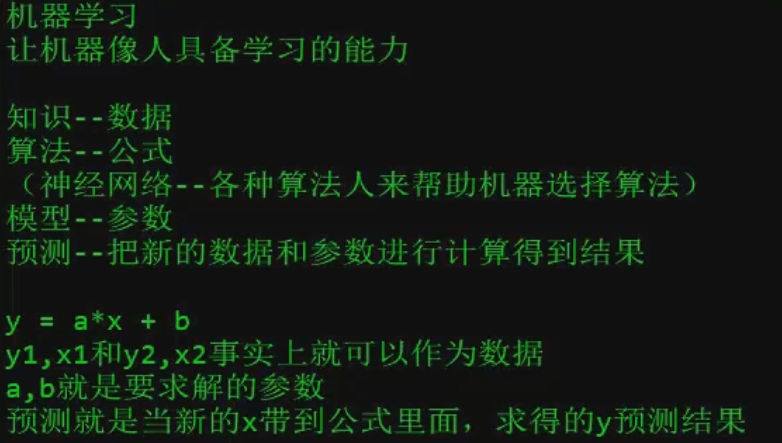
神经网络
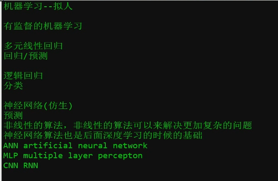

Relu 激活函数 max{0,x}