本文只讨论CNN中的卷积层的结构与计算,不讨论步长、零填充等概念,代码使用keras。
一些名词:
卷积核,别名“过滤器”、“特征提取器”。
特征映射,别名“特征图”。
至于神经元和卷积核在CNN中的区别,可以看参考7(结合参考6)中Lukas Zbinden 写的答案:···“The neuron here represents the dot product of that filter with the input region (omitting bias and activation function here for simplicity)”······“Behind each entry (1x1x1) in the 3D output volume there is a neuron whose weights (i.e. the filter) were multiplied with a part of the input defined by the receptive field of that neuron to produce that entry.” ·····“the neuron in a CNN is only applied to a local spatial region of the input (i.e. its receptive field), not to the entire input as in an MLP. Further, the weights of that neuron are not unique, they are shared between all neurons producing one 2D activation map (i.e. N such maps are equivalent to the aforementioned 3D output volume where N is the number of output channels, i.e. a hyperparameter). Consider the filter that slides over the entire input to produce one such 2D activation map, that is the filter shared among all neurons that participate in producing all the entries making up that 2D activation map.”
准确地说,一个卷积层由一组卷积核组成。
基础卷积操作(参考4):
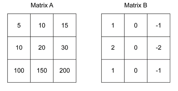
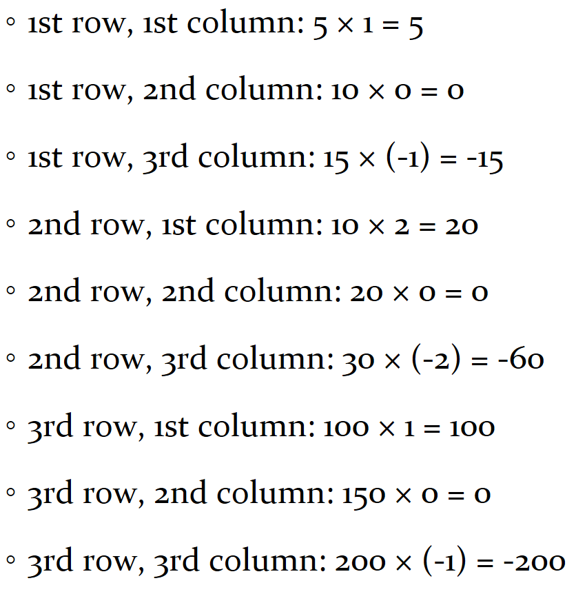
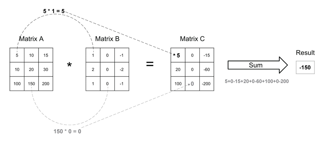
这里的矩阵B就是卷积核,特别地,矩阵B也称作Sobel算子,用于提取垂直特征。
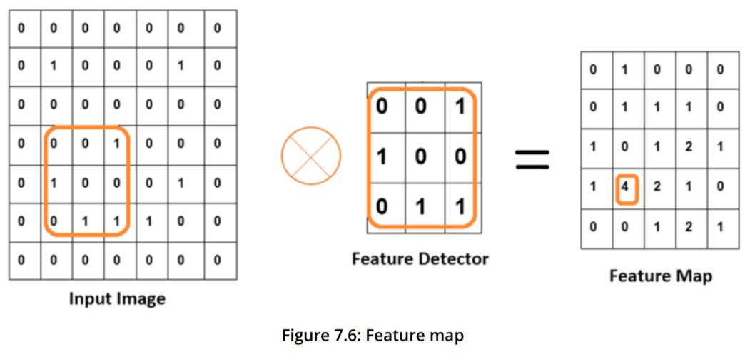
实际上,这里的卷积与图像处理、信号处理中的卷积并不一样,CNN中的卷积是简化了的卷积,又称“互相关”操作。以下引用自参考3:
“在机器学习和图像处理领域,卷积的主要功能是在一个图像(或某种特征) 上滑动一个卷积核(即滤波器),通过卷积操作得到一组新的特征.在计算卷积 的过程中,需要进行卷积核翻转.在具体实现上,一般会以互相关操作来代替卷 积,从而会减少一些不必要的操作或开销.”
而在CNN的卷积层中,我们会在以上的计算(有时也可以再加上一个标量偏置b)之后,使用一个激活函数,以使得CNN具有学习非线性映射的能力。
接下来看一下CNN中卷积层的结构:
用一个卷积核在一个二维图像上进行卷积操作后得到一个二维的特征映射。
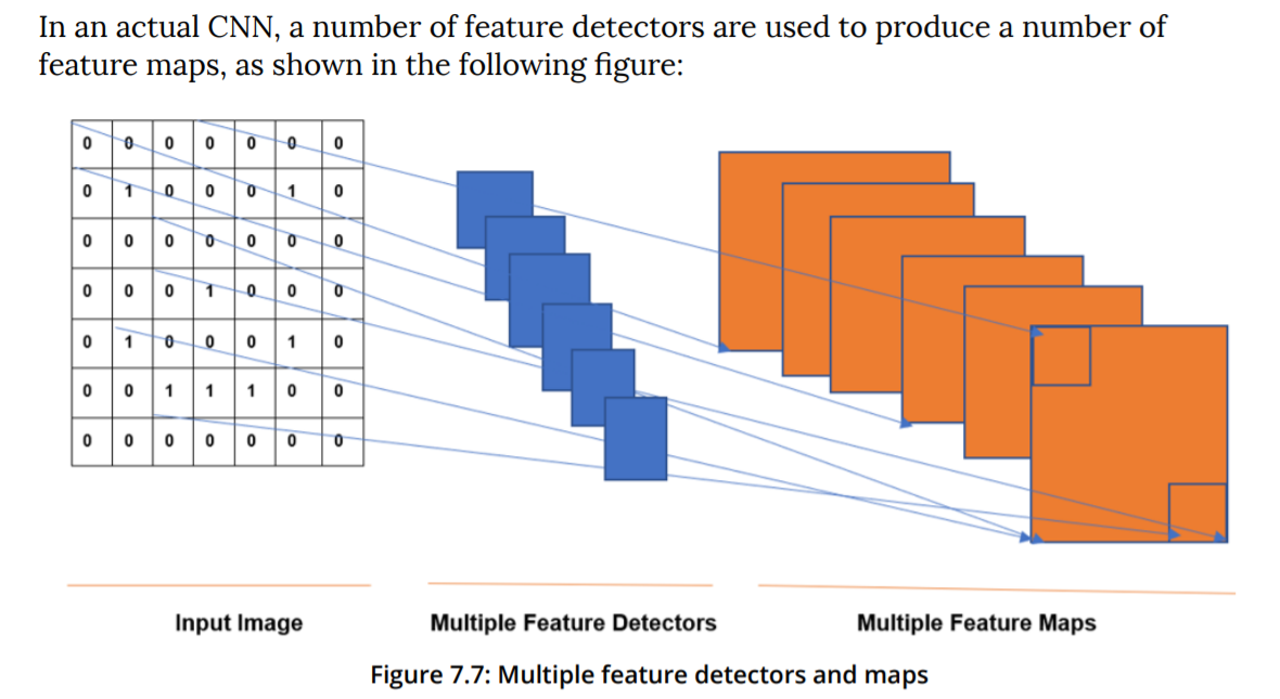
(参考1第230、231页)
(参考2第320页)
通过前两张图可以看出,对于一幅单通道二维图像(M*N)应用某个卷积核(a*a),将得到一个二维的特征映射(M' * N')。而对一幅单通道二维图像(M*N)应用一组卷积核(a*a*D)(一个卷积层)(含有D个不同的卷积核),则得到一组二维特征映射(M' * N' * D)。(假定卷积核是正方形的)
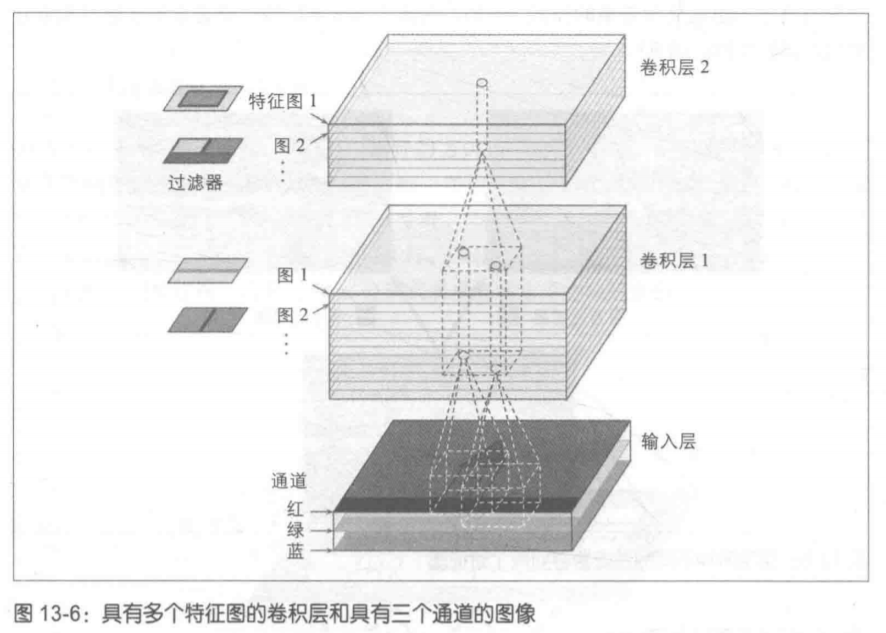
那么如果图像是如上所示的三通道RGB二维图像,经过某个卷积核的卷积操作后,得到的特征映射是什么样的呢?
这里根据:
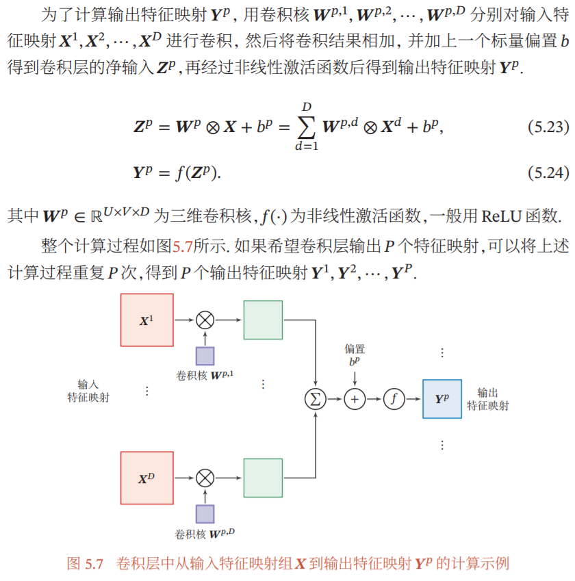
(参考3第113页)(这里作者将激活函数包含于卷积层中)此处输入特征映射xd应该对应于三通道RGB图像中的每个通道,而三维卷积核Wp的概念应该对应于参考5中的说神经元:
“Example 1. For example, suppose that the input volume has size [32x32x3], (e.g. an RGB CIFAR-10 image). If the receptive field (or the filter size) is 5x5, then each neuron in the Conv Layer will have weights to a [5x5x3] region in the input volume, for a total of 5*5*3 = 75 weights”(斯坦福则讲ReLu层分开叙述,实际上是一样的)
参考2第321页
我们可以知道,使用卷积层中的某个卷积核,将其分别作用于图像的三个通道上进行卷积,得到3个子特征映射,再在图像通道维度(3)上相加求和,得到总的特征映射(M' * N' * 3)(可再加上一个标量偏置b)。然后经过一个激活函数,得到最终的特征映射。
(参考5:“The connections are local in space (along width and height), but always full along the entire depth of the input volume.”)
类似地,可以知道,对于处于网络中间的那些卷积层(输入是上一个卷积层的输出特征映射组(M'*N'*d)),他们的卷积操作也是一样的。
下面根据keras代码看一下实际应该怎么写:(参考6)
model = Sequential()
model.add(Conv2D(32, kernel_size=(5, 5), strides=(1, 1),
                 activation='relu',
                 input_shape=input_shape))
model.add(MaxPooling2D(pool_size=(2, 2), strides=(2, 2)))
model.add(Conv2D(64, (5, 5), activation='relu'))
model.add(MaxPooling2D(pool_size=(2, 2)))
model.add(Flatten())
model.add(Dense(1000, activation='relu'))
model.add(Dense(num_classes, activation='softmax'))
对应的网络结构为:
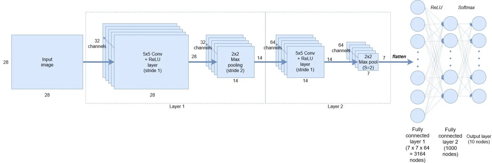
现在便很容易理解Conv2D中的参数了:
model.add(Conv2D(32, kernel_size=(5, 5), strides=(1, 1), activation='relu', input_shape=input_shape))
32即在这个卷积层中使用32个卷积核(过滤器),卷积核尺寸为5*5,横向纵向步长均为1,激活函数为relu。其最终输出的特征映射组的深度也必然是32.
本文为个人学习笔记,如有谬误,敬请指出,谢谢。
参考:
1、The Deep Learning with Keras Workshop: An Interactive Approach to Understanding Deep Learning with Keras, 2nd Edition
2、机器学习实战——基于Scikit-learn和Tensorflow
3、《神经网络与深度学习》邱锡鹏
4、The Deep Learning Workshop: Learn the skills you need to develop your own next-generation deep learning models with TensorFlow and Keras
5、https://cs231n.github.io/convolutional-networks/
6、https://adventuresinmachinelearning.com/keras-tutorial-cnn-11-lines/
7、https://www.quora.com/What-is-a-neuron-in-the-context-of-Convolutional-Neural-Network