期末大作业

一、Boston房价预测

1. 导入boston房价数据集

import numpy
from sklearn.datasets import load_boston
boston = load_boston()
boston.keys()

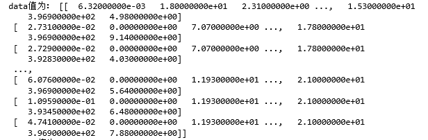
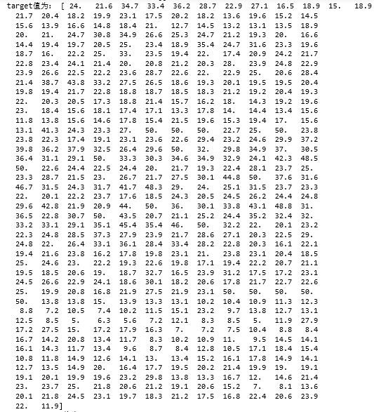
#查看每一个key值#
print('data值为：',boston.data)
print('target值为：',boston.target)
print('feature_names值为：',boston.feature_names)

2. 划分数据集

# 划分数据集
from sklearn.model_selection import train_test_split
x_train, x_test, y_train, y_test = train_test_split(boston.data,boston.target,test_size=0.3)
print(x_train.shape,y_train.shape)

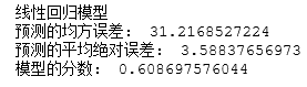
3.线性回归模型：建立13个变量与房价之间的预测模型，并检测模型好坏。

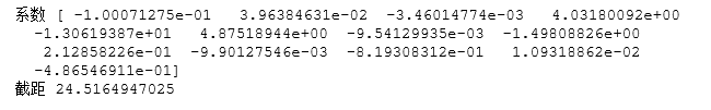
from sklearn.linear_model import LinearRegression
mlr = LinearRegression()
mlr.fit(x_train,y_train)
print('系数',mlr.coef_,"
截距",mlr.intercept_)

from sklearn.metrics import regression
y_predict = mlr.predict(x_test)

print('线性回归模型')
print("预测的均方误差：",regression.mean_squared_error(y_test,y_predict))
print("预测的平均绝对误差：",regression.mean_absolute_error(y_test,y_predict))

print("模型的分数：",mlr.score(x_test,y_test))

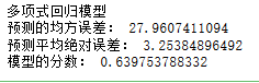
4. 多项式回归模型：建立13个变量与房价之间的预测模型，并检测模型好坏。

from sklearn.preprocessing import PolynomialFeatures
#多项式化
poly2 =PolynomialFeatures(degree=2)
x_poly_train = poly2.fit_transform(x_train)
x_poly_test = poly2.transform(x_test)
#建立模型
mlrp=LinearRegression()
mlrp.fit(x_poly_train,y_train)
#预测
y_predict2 = mlrp.predict(x_poly_test)

print("多项式回归模型")
print("预测的均方误差：",regression.mean_squared_error(y_test,y_predict2))
print("预测平均绝对误差：",regression.mean_absolute_error(y_test,y_predict2))

print("模型的分数：",mlrp.score(x_poly_test,y_test))

5. 比较线性模型与非线性模型的性能，并说明原因。

答：

线性回归模型是一条直线，而多项式模型是一条平滑的曲线，相较之下，曲线更加贴合样本点的分布，并且误差比线性小，所以非线性模型的性能比线性模型的性能更好。

二、中文文本分类

(1) 导包；运用os、walk获取所需变量

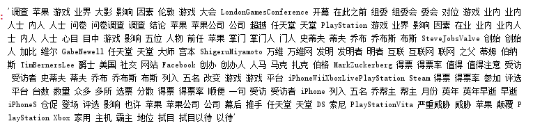
import os
import numpy as np
import sys
from datetime import datetime
import gc
path = 'C:\期末大作业\0369'

#导入结巴库
import jieba
#导入停用词
with open(r'C:\期末大作业\stopsCN.txt',encoding='utf-8') as f:
    stopwords = f.read().split('
')


def processing(tokens):
 
    tokens = "".join([char for char in tokens if char.isalpha()])                    #去掉非字母汉字字符
    tokens = [token for token in jieba.cut(tokens,cut_all=True) if len(token) >=2]   #jieba分词
    tokens = " ".join([token for token in tokens if token not in stopwords])          #去掉停用词
    return tokens


tokenList = []
targetList = []
#通过os、walk获取需要的变量
for root,dirs,files in os.walk(path):
    for f in files:
        filePath = os.path.join(root,f)
        with open(filePath,encoding='utf-8') as f:
            content = f.read()
# 获取新闻类别标签，并处理该新闻
        target = filePath.split('\')[-2]
        targetList.append(target)
        tokenList.append(processing(content))

运行结果：

(2) 划分训练集测试集并建立特征向量,为建立模型做准备

# 划分训练集测试集
from sklearn.feature_extraction.text import TfidfVectorizer
from sklearn.model_selection import train_test_split
from sklearn.naive_bayes import GaussianNB,MultinomialNB
from sklearn.model_selection import cross_val_score
from sklearn.metrics import classification_report
x_train,x_test,y_train,y_test = train_test_split(tokenList,targetList,test_size=0.2,stratify=targetList)
# 转化为特征向量，选择TfidfVectorizer的方式建立特征向量。不同新闻的词语使用会有差别。
vectorizer = TfidfVectorizer()
X_train = vectorizer.fit_transform(x_train)
X_test = vectorizer.transform(x_test)
# 建立模型,这里用多项式朴素贝叶斯，因为样本特征的a分布大部分是多元离散值
mnb = MultinomialNB()
module = mnb.fit(X_train, y_train)

#进行预测
y_predict = module.predict(X_test)
# 输出模型精确度
scores=cross_val_score(mnb,X_test,y_test,cv=5)
print("Accuracy:%.3f"%scores.mean())
# 输出模型评估报告
print("classification_report:
",classification_report(y_predict,y_test))

运行结果：

（3）统计测试集和预测集的各类新闻个数

# 统计测试集和预测集的各类新闻个数
testCount = collections.Counter(y_test)
predCount = collections.Counter(y_predict)
print('实际：',testCount,'
', '预测', predCount)

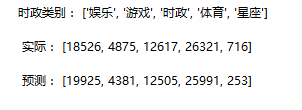
（4）建表分类别

# 建立标签列表，实际结果列表，预测结果列表，
nameList = list(testCount.keys())
testList = list(testCount.values())
predictList = list(predCount.values())
x = list(range(len(nameList)))
print("时政类别：",nameList,'
',"实际：",testList,'
',"预测：",predictList)